power spectral density (PSD). For each frequency ... band power was computed as the sum of all PSD .... bootstrap significance test with 100 permutations [5].
Feature Selection for Brain-Computer Interface N.S. Dias, P.M. Mendes and J.H. Correia Dept. of Industrial Electronics, University of Minho, Campus Azurem, 4800-058 Guimaraes, Portugal Abstract — The implementation of a realistic BrainComputer Interface (BCI) for non-trained subjects requires a classifier able to detect subject-specific electroencephalogram (EEG) patterns. The classifier should be simple enough (i.e. few EEG features, few EEG channels) to enable the mutual adaptation between the BCI and the user. However the classifier should still capture subject-specific EEG patterns. Hence, a feature selection algorithm is introduced as a new method to detect subject-dependent feature and channel relevance for mental task discrimination. This algorithm employs a new formulation of principal component analysis that accommodates the group structure in the dataset. Five subjects were submitted to an EEG experiment that instructed them to perform movement imagery tasks. A linear discriminant classifier used the selected features to discriminate EEG responses to left vs. right hand movement imagery performance with 18% cross-validation error. The discrimination of EEG responses to tongue vs. feet movement imagery performance achieved 26% cross-validation error. Besides the low classification error attained, the selected features often included the frequency-space EEG patterns generally suggested for movement imagery task discrimination. Moreover, each subject’s characteristic EEG patterns were also detected and enhanced classifier performance and customization. Keywords — BCI, EEG, feature selection, PCA.
I. INTRODUCTION Brain-Computer Interface (BCI) enables people to control a device with their brain signals [1]. In a BCI implementation, the electroencephalogram (EEG) channel relevance for mental task discrimination is subject-dependent, specifically when no extensive training sessions are employed. For this reason, a large feature space is usually considered in order to accommodate the high inter-subject variation. However, a classifier trained in a large feature space is likely to suffer of over-fitting. Thus a feature down-selection step should precede the classification process in order to produce a more flexible BCI that still detects the subject performance on different mental tasks. This work introduces a feature selection method, based on a different formulation of principal component analysis (PCA) [2], which accommodates the group structure of the dataset. Five subjects participated on an EEG experiment
that instructed them to perform movement imagery mental tasks. The cross-validation error of the mental task discrimination was calculated to assess the feature selection performance. The subject-specific as well as the generally relevant features were investigated through the feature selection frequency accounted for the cross-validation folds. II. EXPERIMENTAL DESIGN Five healthy human subjects, 25 to 32 years old, four males and one female, none of them under any medication, were submitted to a session of motor imagery tasks. A. Experimental Paradigm Each session had 4 runs of 40 trials each. Each subject was instructed to perform one of 4 tasks in each trial. The tasks were tongue, feet, left hand and right hand movement imageries. The first 2 runs (i.e. 80 trials) of each session cued the subject with 2 different stimuli for imagery performance of either left hand (i.e. arrow pointing leftward) or right hand (i.e. arrow pointing rightward) movements. The last 2 runs (i.e. 80 trials) of each session cued the subject with other 2 stimuli for imagery performance of either tongue protrusion (i.e. arrow pointing upward) or feet (i.e. arrow pointing downward) movement. Each trial started with the presentation of a cross centered on the screen, warning the subject to be prepared. After 3 s, a cue about the required movement imagery (i.e. the arrow pointing to one of the 4 directions) was presented on the top of the cross. The subject was instructed to perform the mental task during the next 4 s. Then, the screen was cleaned out indicating the end of the trial. The inter-trial period was randomly set to 3-4.5 s long. B. Recording Settings Data were acquired from 19 electrodes according to the standard 10-20 system (i.e. Fp1, Fp2, F7, F3, Fz, F4, F8, T7, C3, Cz, C4, T8, P7, P3, Pz, P4, P8, O1 and O2). All electrodes were referenced to linked earlobes. Data were digitized at 256 Hz and passed through a 4th order 0.5-60 Hz band-pass filter. Each channel’s raw EEG signal was epoched from the cue time point to 4 s after the
J. Vander Sloten, P. Verdonck, M. Nyssen, J. Haueisen (Eds.): ECIFMBE 2008, IFMBE Proceedings 22, pp. 318–321, 2008 www.springerlink.com © Springer-Verlag Berlin Heidelberg 2009
Feature Selection for Brain-Computer Interface
319
cue. The presence of artifacts in the epochs was checked through maximum allowed absolute value and maximum allowed absolute potential difference between two consecutive points. The epochs contaminated with artifacts (e.g. eye blinks, muscle artifacts) were excluded from further analyses. Data were re-referenced to common-average in order to improve the spatial resolution. C. Feature Extraction The epoch used to extract the EEG features includes the data from the whole imagery period (i.e. 3 s to 7 s after the trial start). Five frequency narrow bands were defined: 8-12 Hz (i.e. lower alpha band); 10-14 Hz (i.e. higher alpha band); 16-20 Hz (i.e. lower beta band); 18-22 Hz (i.e. mid beta band); and 20-24 Hz (i.e. higher beta band). A frequency broad band was set to 0.5-30 Hz. The time series of each epoch was transformed to the frequency domain by the fast-fourier transform. The dot product of the frequency domain series with its own complex conjugate results in the power spectral density (PSD). For each frequency band, the band power was computed as the sum of all PSD components in the correspondent frequency range. The ratios of the power in the narrow frequency bands to the power in the broad frequency band form the feature vector. In the discrimination context, the feature vectors are grouped per mental task. The feature matrices had 95 columns (i.e. 5 power ratios from each of the 19 electrodes). III. METHODS The introduced feature selection algorithm produces a ranked list of the features extracted from the EEG signals. The original feature matrix Y has samples in rows (n) and features (p) in columns.
AGVi =
vT i Ψ Between vi
(1)
λi
ΨBetween represents the between group covariance matrix [Flury 97] and vi and λi represent respectively the ith eigenvector and correspondent eigenvalue of the total covariance matrix Ψ. The dimensionality reduction results from the truncation of the component matrix (U), whose columns were previously ordered according to the AGV scores. The truncation criterion (δ) is a percentage of the cumulative sum (in descending order of the AGV scores) of every component’s AGV. The algorithm performance was assessed for the following δ values: 60%, 70%, 80% and 90%. The criterion value that achieved the lowest classification error determined the number of components k to retain. The truncated version of U (i.e. Un×k), with k < #pc, is a lower dimensional representation of the original variable space Y. Considering the spectral decomposition property of the covariance matrix, the original k features (Yn×k) with highest variance in the truncated component space (Un×k) correspond to the k highest absolute values in the diagonal of Ψ’ in (2). These k features are used as a low-dimensional representation of the original variable space Y. Therefore, at the end of this stage, the dimensionality of the dataset has been reduced from p to k. k
Ψ ′ = ∑ λi vi viT
(2)
i =1
A. Across-Group Variance (AGV) Algorithm This two-step method uses a different formulation of PCA [3] to reduce data dimensionality in a 1st step. In the 2nd step, the remaining features are ranked according to their discrimination ability. 1) Data Dimensionality Reduction Initially, the principal components (PCs) in Un×#pc (#pc stands for ‘number of PCs’) are calculated through singular value decomposition (SVD) of Y. Although the PCs are already organized by descending order of the total variance, this order is optimized for orthogonality rather than
_________________________________________
discrimination between groups. In order to compensate for this and take the data group structure into account, the components should be ordered according to the across group variance (AGV) score [4] instead. The AGV score in (1) is used to rank each PC in terms of the between group variance instead of the total variance.
2) Feature Ranking In this 2nd step, a ranked list of the retained features is calculated according to their discrimination ability. The score Δj, in (3), computes the multivariate distance penalization observed when the variable j is removed from the subset of k retained variables.
Δ j = D − D− j
IFMBE Proceedings Vol. 22
,
j∈k
(3)
___________________________________________
320
N.S. Dias, P.M. Mendes and J.H. Correia
The multivariate distance D is calculated as in (4). Μ1 and Μ2 are the multivariate means of groups 1 and 2 respectively, and Ψk is the covariance matrix of the k retained variables. D-j is calculated by excluding the variable j to calculate the multivariate distance. T
D = ( Μ1 − Μ 2 ) Ψ k ( Μ1 − Μ 2 )
(4)
The output of this algorithm is a list of the k features retained in the 1st step, ranked in descending order of Δj. B. Linear Discriminant Classifier Once the feature ranked list is calculated, the estimation of an optimal feature subset requires the optimization of the subset size (see subsection D). The size (#opt) of the optimal feature subset, determine how many features from the top of the ranked list should be selected for the optimal feature matrix Yopt. A different approach of Fisher Discriminant Analysis [4] was applied on Yopt according to (5). The canonical discriminant function Z is the result of a linear transformation of Yopt (i.e. the inner product between each feature vector in Yopt and the discrimination coefficient vector bT).
Z = Yopt bT
(5)
Further details on the classification method can be found on previous work [4]. The discrimination quality was assessed through the bootstrap significance test with 100 permutations [5]. C. Cross-Validation Scheme The generalization error used to evaluate the feature selection performance was calculated through a 10-fold double-loop cross-validation (CV) scheme [6]. The performance of the classifier is validated in the 10 folds of the outer loop. However, the classifier needs the parameter #opt to define which features should be selected for training. In the inner loop of the CV scheme, the parameter #opt is optimized on 10 sub-folds of each outer loop fold. Therefore, the CV scheme calculates 10 validation error values of the classifier performance. However the 10-fold CV results are considerably affected by variability. For this reason, the whole CV scheme was repeated 10 times (i.e. 100 validation folds were evaluated) in order to estimate accurately the algorithms’ performance.
_________________________________________
Table 1 Summary results of the generalization classification error and number of features selected. Both left vs. right and tongue vs. feet discriminations were reported for 4 subjects. Subject code
Left vs. Right
Tongue vs. Feet
Error [0-1]
#Features
Error [0-1]
#Features
A
0.14
6
0.25
11
B
0.17
6
0.25
7
C
0.13
5
0.25
9
D
0.29
3
0.29
7
Mean
0.18
5
0.26
9
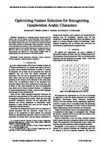
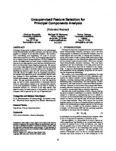
The median error of the 100 validation folds was used to estimate the BCI performance on the selected features (table 1). In order to investigate the channel selection frequency, a counter was assigned to each channel and it was increased each time the channel was selected for validation. Thus, the channels that are highly relevant for discrimination would be selected more frequently then the less relevant channels. Similarly, another counter tracked the frequency band selection frequency. IV. RESULTS The results from one of the 5 subjects tested were excluded from further analyses, since only the other 4 subjects had classification error values that were significant by the bootstrap test. As reported in table 1, the classification error (mean error=0.18) and the number of features selected (i.e. 5 in average) from the left vs. right discrimination were lower than the results achieved for tongue vs. feet discrimination (mean error=0.26 and 9 features selected in average). Therefore only the feature selection frequencies for left vs. right movement imagery discrimination were illustrated on figures 1 and 2. The channel selection frequency on figure 1 shows high inter-subject variation for left vs. right movement imagery discrimination. The Channels C3, C4 and P7 were highly selected for most subjects. The Channels P3, O1 and O2 had high selection frequencies for subject B. The Channel P8 had high selection frequency for subject C and the channel P4 was often selected for subject A. The frequency band selection (figure 2) manifested low inter-subject variation. All 4 subjects had many selections for the frequency band 8-12 Hz (lower alpha). The frequency band 10-14 Hz (higher alpha) was often selected for 3 subjects. The beta frequency bands (i.e. 16-20 Hz, 1822 Hz and 20-24 Hz) were rarely selected for all subjects.
IFMBE Proceedings Vol. 22
___________________________________________
Feature Selection for Brain-Computer Interface
321
Selection Frequency [0-100]
100 Subject A Subject B Subject C Subject D
80 60 40 20 0
Fp1Fp2F7 F3 Fz F4 F8 T7 C3 Cz C4 T8 P7 P3 Pz P4 P8 O1 O2 Channels
Figure 1 Feature selection frequency for 4 subjects per EEG channel. Each individual selection frequency value represents the number of validation folds in which the correspondent channel was selected. The reported results are from the left vs. right discrimination.
Selection frequency [0-100]
100 Subject A Subject B Subject C Subject D
80
relevance and a low subject-dependence of the frequency band relevance. As investigated earlier [8] and confirmed by these results, motor imagery tasks activate primary sensorimotor areas under C3 and C4 locations. Therefore, the channels C3 and C4 were often selected since they represent a frequent spatial pattern for left vs. right hand movement imagery discrimination. The parietal channels (e.g. P7, P3, Pz, P4 or P8) are not selected as frequently for movement imagery discrimination but their relevance has been reported earlier [9]. The frequency band relevance was consistent for all subjects, revealing considerably higher relevance of the alpha rhythms (i.e. 8-12 Hz and 10-14 Hz) than the beta rhythms. The beta rhythms were considered irrelevant for discrimination since the assessed epochs only comprised the performance period, when the alpha rhythm is more reactive than the beta rhythm. In conclusion, the introduced feature selection algorithm succeeded to detect common frequency and spatial EEG patterns on movement imagery task discrimination. Despite of the inter-subject variation, the low classification error values resulted from the detection of subject-specific features that improved classifier customization.
60
ACKNOWLEDGMENT
40
N. S. Dias is supported by the Portuguese Foundation for Science and Technology under Grant SFRH/BD/21529/2005 and Center Algoritmi.
20 0
8-12
10-14 16-20 18-22 Power ratio frequency bands (Hz)
20-24
Figure 2 Feature selection frequency for 4 subjects per frequency band. Each individual selection frequency value represents the number of validation folds in which the correspondent frequency band was selected. The reported results are from the left vs. right discrimination.
1. 2. 3. 4.
V. DISCUSSION AND CONCLUSIONS The classification errors achieved were comparable or even better than others published in the same context [7]. As table 1 show, for each subject, the lowest errors correspond to the smallest feature subsets. The apparent positive correlation between the generalization error and the number of features selected suggests that a smaller proportion of features increases the BCI efficiency and promotes the mutual adaptation between the BCI and the user [7]. The feature selection frequencies reported in the results section manifest a high subject-dependence of the channel
_________________________________________
REFERENCES
5. 6. 7. 8. 9.
Wolpaw J R, McFarland D J and Vaughan T M (2000) Brain– Computer Interface Research at the Wadsworth Center IEEE TRANS. ON REHAB ENG 8 (2):222-226 Jolliffe I T (2002). Principal Component Analysis, Springer. Dillon W R, Mulani N et al. (1989) On the Use of Component Scores in the Presence of Group Structure J. of Consumer Res. 16:106-112 Dias N S, Kamrunnahar M, Mendes P M, Schiff S J, Correia J H (2007) Comparison of EEG Pattern Classification Methods for BrainComputer Interfaces, Proc.29th EMBC, Lyon, France, pp.2540-2543 Flury B (1997) A First Course in Multivariate Statistics. Springer, New York Wessels L F A, Reinders M J T et al. (2005) A protocol for building and evaluating predictors of disease state based on microarray data. Bioinformatics 21(19):3755-3762. Millan J R, Franze M et al. (2002) Relevant EEG features for the classification of spontaneous motor-related tasks. Biol Cybern 86:8985. Pfurtscheller G and Neuper C (1997) Motor imagery activates primary sensorimotor area in humans. Neuros. Letters 239:65-68 Babiloni C, Carducci F et al. (1999) Humana movement-related potentials vs desynchronization of EEG alpha rhythm: a high resolution EEG study. Neuroimage 10:658-665
IFMBE Proceedings Vol. 22
___________________________________________