FFT-based BP Decoding of General LDPC Codes over Abelian Groups. Alban Goupil, Maxime Colas, Guillaume Gelle and David Declercq. AbstractâWe ...
1
FFT-based BP Decoding of General LDPC Codes over Abelian Groups Alban Goupil, Maxime Colas, Guillaume Gelle and David Declercq
Abstract— We introduce a wide class of LDPC codes, large enough to include LDPC codes over finite fields, rings or groups as well as some non-linear codes. A belief propagation decoding procedure with the same complexity as for the decoding of LDPC codes over finite fields is also presented. Moreover, an encoding procedure is developed. Index Terms— Generalized LDPC codes, group, Fourier transform.
I. I NTRODUCTION Since the rediscovery by MacKay [1] of Gallager’s LDPC codes [2], numerous generalizations have been proposed. Among them, the most promising could be roughly divided into two classes. On one hand, irregular binary LDPC codes can be designed to approach capacity. On the other hand, nonbinary LDPC codes have been shown to be very efficient for decoding short to medium length codewords. For example, extensions of LDPC codes over finite fields, rings or groups can be found in [5], [6]. Both approaches have the decoder type in common since Belief Propagation (BP) algorithm (and its simplifications such as min-sum, etc) is generally used as decoder. The BP decoder needs however to be adapted to the specific class of LDPC codes. For instance, for non-binary LDPC codes being defined on higher order finite fields or groups, the BP decoder needs to tackle the dimensionality of the messages, which is greater than one. A description of BP adaptations for LDPC codes over GF(2p ) can be found in [7] and [8]. In this paper, we propose a further generalization of the nonbinary LDPC codes. And its contribution is two-fold. First, in Section II, we show that it is sufficient to consider a group as the underlying algebraic structure of a LDPC code. This allows one to consider general parity equations by combining any mapping acting upon the considered group. Secondly, the other important point of our work is that the generalization of the parity equations does not overweight the BP decoding complexity. Indeed, Section III shows that the adaptation of the BP algorithm for the general parity check is as complex as the one used for decoding LDPC codes over GF(q). Section IV is concerned specifically with the encoding problem. Finally, a simulation example, using a method described in Section V, is presented in Section VI. Conclusions are drawn in Section VII. II. G ENERAL NON - BINARY LDPC CODES Classically, LDPC codes are described, thanks to the local constraints given by a parity check relation over some of the
variables (codeword symbols) vi . If they are linear over a finite field GF(q), the parity equations are of the form X hi vi ≡ 0 in GF(q). (1) i
The additive law in (1) remains primordial because it defines the local constraint of the code. The multiplicative law is however excessive because the constraints do not involve the distributivity of multiplication over addition. This remark leads us to generalize (1). Let G be an Abelian group and the codeword symbols take their values in G. Let also hi be arbitrary mappings from G to G. Notice that hi are not necessarily homomorphisms. We define the following parity equation in a very general sense: X hi (vi ) ≡ 0 in G. (2) i
The generality of this kind of parity check (2) leads to two main advantages, i.e., from the group G’s point of view and from the set A of non-zero mappings hi . • Parity equation of type (2) is general enough to be able to represent linear codes over any rings R like Zq or field GF(q). The group G is simply the additive group of R, (R, +), and the set A becomes the set of all multiplications by a non-zero element of R. Thus the following BP-algorithm becomes practicable for these codes once an efficient FFT over G is available. Some non-linear codes over GF(q) are linear over Zq and hence are more manageable for encoding over Zq than their GF(q) counterpart. For example, it is well known that some pretty good codes over the ring Z4 , like the Nordstrom-Robinson code, can be non-linear over the fields GF(2p ) [9], [10], [11]. The parity in (2) is general enough to represent these kind of codes by using the additive group of Z4 . Thus, (2) is flexible enough to manage different representations of a same code and the BP-decoding algorithm is directly accessible from the rest of the paper. • The first point deals with the underlying group G to represent a code in the most manageable way. But the parity (2) can also be used to extend the search-space of LDPC. In fact the set A is not constraint in (2) and can be any subset of the set of mappings over G. In fact the size of A is greatly enlarged. Compare its size for linear codes over a field GF(q) or a ring Zq and the size of all non-zero applications over a group of size q: only q − 1 applications are possible in the former case whereas q q − 1 arbitrary mappings can be chosen
2
in the latter. Even if the set A is restricted to contain only permutations over G, its size is still huge, that is q!. Further, if we wish to have some kind of linearity, that is, say G is a R-module, where R is a ring of size p, there are around q p linear operators available for A, where q is the size of G. These extensions may be useful. Indeed, sometimes, the group structure is given by the application —to match the channel, for example, [12]— and using (2), we can derive LDPC codes by fixing the set A of “good” mappings over G. Another interest of this generality will be derived in Section V where, via bit-clustering, the trade-off between decoding complexity and decoding performance becomes tunable. However, the size of A may be problematic because one does not have linearity of the code and thus the encoding should be addressed for each individual construction. However in Section IV, a procedure is given for encoding which works in some cases. Any finite group G of order q would fit to define a general non-binary parity code with equations (2). However, the group choice is also governed by the decoding complexity. In fact, the BP decoding algorithm described in the next section has the same complexity as the BP decoding of linear LDPC over GF(q), based on the assumption that the group G has a fast Fourier transform. That is the case for the most interesting groups like Z2p and Zp2 , but not for some other groups. In the sequel, we will restrict the discussion to those groups which admit a fast Fourier transform, leading to a reasonable decoding complexity. III. B ELIEF P ROPAGATION DECODING OF GENERAL LDPC CODES
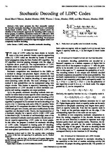
A. Algorithm and complexity BP algorithm propagates messages between the nodes of the factor graph of the code. As the factor graph of LDPC codes are bipartite, there are two kind of messages: from check nodes to variables nodes and from variables nodes to checks nodes. In our case, the messages are represented as an array indexed by group elements. For example µ(g) means: the complex value of the message/array µ indexed by the group element g ∈ G. The implementation of BP algorithm is made of two passes: data pass and check pass. The former is the simpler since it does not involve labels. Consider the computation of the message µ sent by the variable node v to the check node c. The neighbors of v are c and ci for i = 1, . . . , d. Extrinsic principle implies that µ depends only on incoming messages from ci and on the message µch from the channel. Notations are given on Fig. 1. The computation of the message µ during the data pass consists of the term-by-term product of the incoming messages µ(g) = µch (g)
d Y i=1
µi (g) ∀g ∈ G,
(3)
µch c1 µ1 v
µ
c
µd cd Fig. 1.
Messages at a variable node.
However, the check pass is more complicated as it involves the edge’s labels. Consider the parity equation (2) and the resulting graph in Fig. 2. v1 µ1 h1 hd
c
µ h
v
µd
vd Fig. 2.
Messages and labels at a check node.
The message µ sent by the check node c to the variable node v depends on the incoming messages µi from neighbors vi , for i = 1, . . . , d and on their associated label hi and on the label h. Fig. 2 is therefore the graphical representation of the parity check equation h(v) +
d X
hi (vi ) ≡ 0
in G.
(4)
i=1
As the group G is Abelian, there exists a Fourier transform F. The next subsection will prove that the computation of a message µ during the check pass can be performed using the relation, d �Y �� � µ(x) ∝ F −1 F ∗ µhi i h(x) , (5) i=1
where µhi i (y) =
X
µi (x).
(6)
x∈h−1 i ({y})
If, moreover, the Fourier transform can be computed efficiently by a FFT, the preceding equation gives directly the following algorithm: 0 1 2 3 4 5 6 7
require µ01 (g) = · · · = µ0d (g) = µ(g) = 0 ∀g ∈ G for i = 1, . . . , d do for g ∈ G do µ0i (hi (g)) ← µ0i (hi (g)) + µi (g) done µ0i ← FFT∗ (µ0i ) done Qd for g ∈ G do µ0 (g) ← i=1 µ0i (g) done µ0 ← IFFT(µ0 ) for g ∈ G do µ(g) ← µ0 (h(g)) done
The complete check pass consists thereafter to perform this algorithm for each check node. Note that the ∗ in line 3 that indicates complex conjugate. The complexity of the FFT/IFFT pair or special implementation tricks of the previous algorithm make the complexity
3
analysis difficult. However, using the big-O notation, the main result of this paper is highlighted. An iteration of the BP decoder is divided into one data pass and one check pass. The data pass has complexity O(eq) where e is the number of edges in the factor graph and q is the size of the group G.� Moreover the complexity of the check pass is O e(5q + 2fq ) where fq is the complexity of the FFT/IFFT. Classically, fq is O(q log q) for most interesting groups. Thus, the complexity of one iteration of the BP decoder is O(eq log q). However, if the FFT/IFFT approach is not used, the complexity reaches O(eq 2 ) which is prohibitory when the size q of the alphabet is large. Remark that the improvement between both algorithms is the same as between brute force Fourier transform and its fast version. The algorithm relies heavily on the FFT/IFFT pair. Therefore groups G in (2) should be carefully chosen. The group (Zp2 , +) which is the additive group of GF(2p ) is one of the most interesting one because the FFT is simply the fast Hadamard transform and consists only of additions and subtractions, making the algorithm even faster. Other groups of interest are Z2p or Zn where n factors into small primes. For all these groups, FFT can be computed in O(q log q), see, for example, the library FFTW [13]. Let us compare this algorithm and the one used for LDPC over GF(q) as developed in [7] or [8]. For all algorithms, the data passes are exactly the sames. However, for the check pass, we can simplify the previous algorithm to obtain the GF(q) version. The differences are in lines 2 and 7 which should be replaced by: 2’
.. . 7’
for g ∈ G do µ0i (hi · g) ← µi (g) done
the check pass is concerned, because during the data pass, the message update rule remains (3). The Fourier transform approach comes directly from the fact that the updating rule in check pass involves convolution, not over a field but over a group. Before this derivation, let us recall some aspects of the Fourier transform over groups. Let χ be a character of G, that is, a homomorphism between G and the multiplicative group of the complex field C. All the b whose size is the same characters of G form a group noted G as that of G. This group is a basis of the space of all functions from G to C. So, a mapping f : G → C can be decomposed as X f (x) = fb(χ) χ−1 (x), (7) b χ∈G
where the coefficients fb(χ) are given by the Fourier transform over the group G, 1 X fb(χ) = f (x) χ(x). (8) |G| x∈G
As in the complex case, where the characters are given by complex exponential, the computation of the transform (8) can be done with small complexity thanks to fast algorithms for groups of interest, i.e., Zp2 and Z2p . Note also that, as χ is an homomorphism, χ−1 (x) = χ(−x) = χ∗ (x). For notational convenience, fb(χ) will be written F(f )(χ), that allows us to use F(f ) which means the complete Fourier transform of the function f and to use F −1 for the inverse transform. b has also another nice property: it is an The group G orthogonal basis, and so, we have the identity: X χ(x) = |G| · [x ≡ 0 in G] , (9)
for g ∈ G do µ(g) ← µ0 (h · g) done
where hi , for i = 1, . . . , d, and h are elements of GF(q) and · is the multiplication of elements of GF(q). Moreover, as the multiplication by a non-zero element is a permutation of GF(q), the requirement given by line 0 is not needed anymore. The FFT over GF(2p ) is the same as the FFT over Zp2 , that’s why we claim that both algorithms share the same complexity. When the set of the labels hi is constraint, the algorithm could be improved. For example if hi is a permutation, like in GF(q) case, there is no need to initialize the message µ0i to 0. Moreover, the action of the permutations performed in line 2 and 7 can be computed fast using the decomposition of the permutation into cycles. In this case, in-place replacements allow us to remove the temporary arrays µ0 and µ0i . Moreover, as the messages µ between nodes are real arrays, the computations can be done in the real numbers field R and not in C by using Hartley transforms in place of Fourier transform. But its superiority over the FFT is not significant unless memory space becomes critical. B. Derivation of the algorithm As a Fourier transform can be defined over all finite Abelian group, an FT-based decoding algorithm for the general LDPC given by (2) can be derived in the same way as for LDPC codes over GF(q). As said in the previous section, only
b χ∈G
where [P ] is the indicator function of P , i.e., [P ] = 1 if the proposition P is true, 0 otherwise. According to the above mentioned properties, we can compute the message update through check nodes. Let µi be the i-th incoming message to the check node coming from symbol node vi , for i = 1, 2, . . . , d. Let µ be the output of the check node computation, as was shown in Fig. 2. The extrinsic message µ is the marginalization of the incoming messages [14], [15], µ(x) =
Xh
h(x) +
x1 ∈G ... xd ∈G
d X
d iY
hi (xi ) ≡ 0
i=1
µi (xi ),
(10)
i=1
where the operations in the brackets are done using the additive law of the group G. Notice that the messages are probabilities P and are subjects to the constraints µ(x) = 1. So, x∈G only proportions between the values of µ(x) are of interest. That is why we do not take the proportion coefficient under consideration. Using the relation (9), the preceding equation becomes d d �Y X X X � µ(x) ∝ χ h(x) + hi (xi ) µi (xi ). (11) x1 ∈G χ∈G b ... xd ∈G
i=1
i=1
4
Notice that the argument of χ involves group additions and not complex or real ones. Since χ is a homomorphism, i.e. χ(a + b) = χ(a)χ(b), the expansion of the argument of χ in (11) gives us µ(x) ∝
d d �Y �Y χ h(x) χ hi (xi ) µi (xi ).
X X x1 ∈G χ∈G b ... xd ∈G
i=1
(12)
i=1
Factorizing the last relation and relabeling the indices, relation (12) can be rewritten as µ(x) ∝
X
d X �Y � χ h(x) χ hi (x0 ) µi (x0 ).
(13)
i=1 x0 ∈G
b χ∈G
The aim of the next calculation is to link the inner sum of (13) with the Fourier transform of µi . Denoting S as this sum and by removing the index i in order to simplify the notation, we get X S= χ h(x))µ(x). (14) x∈G
Being a mapping, h uniquely associates x with h(x) and thus P y [y = h(x)] = 1. The sum S can be therefore rewritten X X� � � S= χ h(x) µ(x) y = h(x) (15) x∈G
=
y∈G
�X � �� χ(y) µ(x) y = h(x) .
X y∈G
(16)
x∈G
µ(x) ∝
d �Y � χ h(x) F µhi i (χ),
which is the inverse Fourier transform of the the computation is done by µ(x) ∝ F −1
d �Y
� where ◦ is the composition, i.e., f ◦ g(x) = f g(x) . For the rest of paper, the construction [A, B] means the matrix obtained by appending the columns of B to those of A. First assume that, after row and column permutations, the parity matrix H of size m × n can be written in the form [L · U, B]. where L is a lower triangular square-matrix of size m × m filled with endomorphisms of G, the group formed by the mappings G → G respecting the addition in G and denoted End(G). And the diagonal of L contains only the identity map. U is an upper-triangular square-matrix of size m × m filled with mappings and where the mappings on the diagonal are invertible. Once H is given in the previous form then an encoding procedure is performed by p = U−1 L−1 (−Bs) where s is the information vector of size n − m and p is the corresponding redundancy vector of size m. The codeword is then the concatenation [p, s]. These computations are done by the following algorithm where additions/subtractions and equality concern the group G. 0
F ∗ µhi i
��
Q
(17)
factor. In fact,
� h(x) ,
2 3 4 5 6 7 8 9
i=1
b χ∈G
k
1
The sum in parenthesis is a function of y that we denote as µh (y). The sum S in (16) clearly� involves the Fourier transform of µh (y), that is, S = F µh (χ). The P computation of µh h from µ is simple because we have µ (y) = x∈h−1 ({y}) µ(x) where h−1 ({y}) is the set of the antecedents of x under h. Finally, using the preceding S calculation, the message (13) can be computed by X
As the non-zero entries of the check matrix H are not elements of a commutative ring, careful use of matrices is concerned. Given two matrices A and B, the product C = A · B is defined by X ci,j (x) = ai,k ◦ bk,j (x), (19)
(18)
i=1
Practically, the above updating rule is implemented using the algorithm presented in Section III-A.
10
Inversions of L and U are done via forward and backward substitutions, respectively at lines 4–6 and 7–10 and can easily be done on-line. In order to transform the check matrix H into the form [U · L, B], we have slightly modified the classical LU decomposition algorithm to take into account the non-square aspect of H and its elements. The algorithm below gives the procedure to follow in order to achieve this task. 1
IV. E NCODING The encoding procedure of LDPC codes is difficult to obtain in general. When the parity equations are extended into equation (2), this task becomes much harder. But using ideas from binary LDPC codes or over GF(q) exposed in [16], [17], we can give a general, yet simple, procedure to encode general LDPC codes defined by (2). However, the algorithm presented below does not work for all cases and does not solve the encoding problem in general. But, from the tests we have done, this algorithm is good enough for majority of the cases.
require p1 ≡ . . . ≡ pn ≡ 0 for k = 1, . . . , m do for i = 1, . . . , n − m do pk ← pk − bk,i (si ) done done for k = 1, . . . , m do for i = 1, . . . , k − 1 do pk ← pk − lk,i (pi ) done done for k = m, . . . , 1 do for i = k + 1, . . . , m do pk ← pk − uk,i (pi ) done pk ← u−1 k,k (pk ) done
2 3 4 5 6 7 8 9
for k = 1, . . . , m do Find an invertible pivot hr,c , r, c ≥ k such that hi,c ◦ h−1 r,c ∈ End(G) for i ≥ k Swap rows r and k and columns c and k in H for i = k + 1, . . . , m do hi,k ← hi,k ◦ h−1 k,k done for i = k + 1, . . . , m do for j = k + 1, . . . , m do hi,j ← hi,k ◦ hk,j done done done
At the end of this procedure, the first square part of the matrix H contains L − I + U, and thus L and U can be easily
5
V. B IT CLUSTERING As an illustration of these generalized LDPC codes, let us now describe a simple construction, called bit clustering, that will be needed in the next section to serve as an example. The elements of the group G = Zp2 are binary vectors of length p which are alternatively represented as decimal numbers, wherein the first bit of the binary vector is taken to be the most significant bit for the decimal number. For example, in Z42 , the binary vector [1, 1, 0, 1] is the element 13 in G. Given the n × m parity check matrix of a binary code, p codeword bits are grouped together to form a symbol of the group G = Zp2 . So, the binary check matrix can be represented as a n/p × m/p matrix whose parity check equations are of the form (2). Consider for example the systematic check matrix of the extended Hamming code [8, 4, 4] 1 0 0 0 0 1 1 1 0 1 0 0 1 0 1 1 H= (20) 0 0 1 0 1 1 0 1 0 0 0 1 1 1 1 0 and regroup the codeword bits two by two in natural order. The resulting matrix is given by � � 1 0 a b H2 = (21) 0 1 b a where 1 is the identity of G, a is the transposition (1 2) and b maps 1 and 2 to 3 and maps to 0 otherwise. Notice that b is not a permutation of the group, but the generality of (2) allows us to consider this kind of function. In this case, we could expect a better BP decoding behavior using (21) rather than (20) because the number of cycles in the factor graph is reduced and the local decoding takes more information into account. Furthermore, bit clustering can be done four by four to get the matrix H4 = [1 c] over the group Z42 , where c is
the permutation (1 14)(2 13)(4 11)(7 8). So, in this form the corresponding factor graph becomes a very simple tree: a single edge and two leaves. Consequently, BP algorithm is optimal on this factor graph. Thus, the idea behind bit clustering is to use the BP decoding algorithm on sparser graphs to get better performance. With this technique, trade-offs between decoding complexity and decoding performance can be achieved. VI. E XAMPLES A. Bit clustering of QR[48,24,12] code In this section, we illustrate the use of the general LDPC and its decoding algorithm using an example based on the bit clustering construction described in the Section V. It involves a classical extended QR code [48, 24], whose parity check matrix is taken in systematic form and the bits are regrouped two by two, four by four, and so on until, twelve by twelve. The corresponding matrices get smaller from 48 × 24 to 2 × 4. The mappings related to the regrouping are then computed; the chosen group G is therefore Z2p for p = 1, . . . , 12. Notice that in these extensions, the mappings are no longer linear operators over the field GF(2p ) and even some of them are not permutations. The corresponding simulation results over AWGN channel with BPSK modulation are given in Fig. 3. We have plotted word error rate against signal-to-noise ratio. The BP algorithm is iterated 10 times but if during the iterations, the hard-decision word belongs to the code, it is output. 100
10−1
10−2 WER
obtained, and the n − m last columns of the permuted initial matrix H gives B. The condition on the pivot in line 3 ensures that the matrix L is filled with endomorphisms. In order to retain the sparseness of H, and thus the sparseness of L and U, the choice of the pivot is crucial. As it is not fixed completely by the above procedure, an easy way to do it consists in choosing the pivot within the columns with minimal number of non-zero values after the row k. Other pivoting strategies are however possible as described in [17]. The encoding can also be done by other means like choosing a matrix H in a systematic form, or by adapting the algorithm given in [18]. It should be mentioned that the preceding procedure can fail because no pivot is found. It does not mean that no encoding is possible but that others techniques should be used. Indeed, this case could also happen in the linear case when the matrix H is not full rank. Note that the condition of line 3 is always satisfied in the case of LDPC codes over GF(q) and in this context, an “invertible pivot” means a non-zero element of GF(q).
MLD 10−3
10−4
10−5
Z22
Z12 2 Z82 0
2
4
6
Z62 8
Z42
Z2 10
12
Eb /N0
Fig. 3. Performances of extended QR [48, 24] on the AWGN channel for different group order.
As the decoding of parity checks is more global when the extension degree grows, the decoding performance gets better. In fact when the bits of codewords are grouped by twelve, the factor graph [ 10 01 ac db ] is so simple that the decoding is quasioptimal, i.e. close to the maximum likelihood decoding (MLD on Fig. 3), because it contains only one cycle. This example shows clearly that using the regrouping of bits and thanks to the formalism described in this paper, we are able to reach very good performance for short codeword length, and with a reasonable decoding complexity.
6
B. Hamming codes over Z2p As a second example, we will deal with codes defined directly over the group Z2p and not by bit clustering. In [19], the authors “lift” the extended binary Hamming code to the 2-adic Hamming codes H∞ whose generator matrix is 1 λ λ−1 −1 1 1 λ λ−1 −1 1 , (22) 1 λ λ−1 −1 1 1 λ λ − 1 −1 1 where λ is a 2-adic number that satisfies λ2 − λ + 2 = 0, that is λ = 0 + 2 + 4 + 32 + 128 + 256 + · · · . From the self-dual code H∞ , we can get several codes H2p by projecting H∞ over the ring Z2p . These codes are not necessary linear over the binary field. For example, H4 is the octacode which is equivalent to the binary non-linear Nordstrom-Robinson code under the Gray mapping. Using the parity check matrix (22), we simulate the codes H2 , H8 , H32 , and H128 over the AWGN channel with BPSK. The mapping between bits and elements of Z2p is the Gray one in order to increase the minimal Lee distance as shown in [19]. The bit error rates for these codes using the BP decoder are plotted against SNR on the Fig. 4. The BP decoder uses the same stopping rules as above, that is, a maximum of 20 iterations is performed unless a codeword is found before.
10−1
BER
10−2
10−3 Z2 10−4 Z27 Z23 Z25
10−5 0
2
4 Eb /N0
6
8
Fig. 4. Performances of some extended Hamming codes over rings Z2p on the AWGN channel.
Note that the parity check matrix (22) creates a bipartite graph which contains numerous (25) 4-cycles. Thus the algorithm is far from optimal. But as shown in the previous section, we can cluster bits together in order to remove 4-cycles and thus improve performances at the cost of small complexity increase. Results indicate that, without changing the structure of the code, extensions are done easily and performance increases with them. This fact highlights the interest of our construction. VII. C ONCLUSION We introduced in this paper a generalization of LDPC codes. This generalization is achieved through the use algebraic group
structure in parity check constraints. The codes derived from these check equations can be either linear or non-linear. Using Fourier transform over groups, a BP decoding algorithm was proposed for LDPC codes whose check nodes correspond to the general parity constraints. In addition an encoding procedure was described to show the effectiveness of this new class of LDPC codes. As an example, a bit clustering construction based on classical binary codes was presented that highlights the potential of our approach in terms of performance/complexity trade-off. Finally, we think that the general parities defined in this paper open some new perspectives in LDPC code construction due to the increased number of possible mappings hi . R EFERENCES [1] D. J. C. MacKay, “Good error-correcting codes based on very sparse matrices,” IEEE Trans. Inform. Theory, vol. 45, no. 2, pp. 399–431, Mar. 1999. [2] R. G. Gallager, Low density parity check codes. M.I.T press, 1963. [3] M. G. Luby, M. Mitzenmacher, M. A. Shokrollahi, and D. A. Spielman, “Analysis of low density codes and improved designs using irregular graphs,” in Proceedings of 30th ACM STOC, May 1998. [4] ——, “Improved low-density parity-check codes using irregular graphs,” IEEE Trans. Inform. Theory, vol. 47, no. 2, pp. 585–598, Feb. 2001. [5] M. C. Davey and D. J. C. MacKay, “Low density parity check codes over GF(q),” IEEE Commun. Lett., vol. 2, no. 6, June 1998. [6] D. Sridhara and T. E. Fuja, “Low density parity check codes over groups and rings,” in Proceedings of ITW2002, Bangalore, India, Oct. 2002. [7] M. C. Davey, “Error-correction using low-density parity-check codes,” Ph.D. dissertation, University of Cambridge, Dec. 1999. [8] D. Declercq and M. Fossorier, “Decoding algorithms for LDPC codes over GF(q),” submitted to IEEE Trans. Commun., March 2005, second stage revision. [9] A. R. Hammons, Jr., P. V. Kumar, A. R. Calderbank, N. J. A. Sloane, and P. Sol´e, “The Z4-linearity of Kerdock, Preparata, Goethals, and related codes,” IEEE Trans. Inform. Theory, vol. 40, no. 2, pp. 301–319, Mar. 1994. [10] V. S. Pless and Z. Qian, “Cyclic codes and quadratic residue codes over Z4,” IEEE Trans. Inform. Theory, vol. 42, no. 5, pp. 1594–1600, Sept. 1996. [11] J. Wolfmann, “Binary images of cyclic codes over Z4,” IEEE Trans. Inform. Theory, vol. 47, no. 5, pp. 1773–1779, July 2001. [12] A. Bennatan and D. Burshtein, “On the application of LDPC codes to arbitrary discrete-memoryless channels,” IEEE Trans. Inform. Theory, vol. 50, no. 3, pp. 417–438, Mar. 2004. [13] “Fastest Fourier transform in the West,” http://www.fftw.org/. [14] F. R. Kschischang, B. J. Frey, and H.-A. Loeglier, “Factor graphs and the sum-product algorithm,” IEEE Trans. Inform. Theory, vol. 47, no. 2, pp. 498–519, Feb. 2001. [15] S. M. Aji and R. J. McEliece, “The generalized distributive law,” IEEE Trans. Inform. Theory, vol. 46, no. 2, pp. 325–343, Mar. 2000. [16] Y. Kaji, M. P. Fossorier, and S. Lin, “Encoding LDPC codes using the triangular factorization,” in Proceedings of ISITA’04, Parma, Italia, Oct. 2004. [17] R. M. Neal, “Sparse matrix methods and probabilistic inference algorithms,” in IMA program on codes, systems and graphical models, 1999. [18] T. J. Richardson and R. L. Urbanke, “Efficient encoding of low-density parity-check codes,” IEEE Trans. Inform. Theory, vol. 47, no. 2, pp. 638–656, Feb. 2001. [19] A. R. Calderbank and N. J. A. Sloane, “Modular and p-adic cyclic codes,” Designs, Codes and Cryptography, vol. 6, no. 1, pp. 21–35, July 1995.