Filtering Large Propositional Rule Sets While ... - Semantic Scholar

Filtering Large Propositional Rule Sets While Retaining Classifier Performance Siv. ing. (MSc) Thesis

˚ Thomas Agotnes Knowledge Systems Group Department of Computer and Information Science Norwegian University of Science and Technology

February 18, 1999

It is vain to do with more what can be done with less William of Occam

Abstract Data mining is the problem of inducing models from data. Models have both a descriptive and a predictive aspect. Descriptive models can be inspected and used for knowledge discovery. Models consisting of decision rules – such as those produced by methods from Pawlak’s rough set theory – are in principle descriptive, but in practice the induced models are too large to be inspected. In this thesis, extracting descriptive models from already induced complex models is considered. According to the principle of Occam’s razor, the simplest of two models both consistent with the observed data should be chosen. A descriptive model can be found by simplifying a complex model while retaining predictive performance. The approach taken in this thesis is rule filtering; post-pruning of complete rules from a model. Two methods for finding high-performance subsets of a set of rules are investigated. The first is to use a genetic algorithm to search the space of subsets. The second method is to create an ordering of a rule set by sorting the rules according to a quality measure for individual rules. Subsets with a particular cardinality and expected good predictive performance can then be constructed by taking the first rules in the ordering. Algorithms for the two methods have been implemented and is available for general use in the R OSETTA system, a toolkit for data analysis within the framework of rough set theory. Predictive performance is estimated using ROC analysis, and ten different formulas from the literature that can be used to define rule quality are implemented. An extensive experiment on a real-world data set describing patients with suspected acute appendicitis is included. In this study, rule sets consisting of six to twelve rules with no significantly different estimated predictive performance compared to full models consisting of between 400 and 500 rules were found. Another experiment confirms these results. In the experiments, statistical hypothesis testing was used to assert difference between performance measures derived from ROC analysis.

Acknowledgments The work in this thesis has been done in a stimulating research environment in the Knowledge Systems Group. First of all, I would like to thank my supervisor Aleksander Øhrn for his time, guidance and advice, and especially for providing the R OSETTA library. Thanks to Professor Jan Komorowski for advise, discussions and support. Thanks to Terje Løken and Tor-Kristian Jenssen for general discussions and much needed coffee breaks, and especially to Terje for – often long and heated – discussions regarding rough sets, classification and statistical hypothesis testing. Thanks to Staal Vinterbo for providing his genetic algorithm implementation, and for enthusiasm and encouragement in the early phases. Thanks to Turid Follestad for a discussion about statistical hypothesis testing, and to Keith Downing for advise regarding genetic algorithms. Thanks to Grethe Røed for commenting on a draft version of this document. I would also like to thank those who made the experiments possible; Ulf Carlin for doing the initial analysis of the acute appendicitis data, Stein Halland et. al. for providing the acute appendicitis data, and Robert Detrano for providing the Cleveland data set. Finally, thanks to my wife Cecilie for her support and understanding, especially during the last hectic weeks.

Contents Acknowledgments 1

vii

Introduction 1.1 Knowledge Discovery in Databases . 1.2 Model Representation . . . . . . . . 1.2.1 Rule-based Models . . . . . . 1.3 Motivation . . . . . . . . . . . . . . . 1.3.1 Rule Pruning . . . . . . . . . 1.3.2 Finding Submodels . . . . . . 1.4 Research Methodology and Results . 1.5 Related Work . . . . . . . . . . . . . 1.5.1 Pruning . . . . . . . . . . . . 1.5.2 Rough Set Approaches . . . . 1.6 Overview . . . . . . . . . . . . . . . .

. . . . . . . . . . .

. . . . . . . . . . .

. . . . . . . . . . .

. . . . . . . . . . .

. . . . . . . . . . .

. . . . . . . . . . .

. . . . . . . . . . .

. . . . . . . . . . .

. . . . . . . . . . .

. . . . . . . . . . .

. . . . . . . . . . .

. . . . . . . . . . .

. . . . . . . . . . .

. . . . . . . . . . .

. . . . . . . . . . .

. . . . . . . . . . .

. . . . . . . . . . .

. . . . . . . . . . .

. . . . . . . . . . .

I Background 2

3

4

Information and Discernibility 2.1 Introduction . . . . . . . . . 2.2 Knowledge . . . . . . . . . . 2.3 Information Systems . . . . 2.3.1 Discretization . . . . 2.4 Discernibility . . . . . . . . 2.5 Reducts . . . . . . . . . . . . 2.5.1 Dynamic Reducts . . 2.6 Classifiers . . . . . . . . . . 2.6.1 Binary Classification

1 1 2 2 2 3 3 4 4 4 5 5

7 . . . . . . . . .

. . . . . . . . .

. . . . . . . . .

. . . . . . . . .

. . . . . . . . .

. . . . . . . . .

. . . . . . . . .

. . . . . . . . .

. . . . . . . . .

. . . . . . . . .

. . . . . . . . .

. . . . . . . . .

. . . . . . . . .

. . . . . . . . .

. . . . . . . . .

. . . . . . . . .

. . . . . . . . .

. . . . . . . . .

. . . . . . . . .

. . . . . . . . .

. . . . . . . . .

. . . . . . . . .

. . . . . . . . .

9 9 10 11 12 12 14 14 15 16

Propositional Decision Rules 3.1 Introduction . . . . . . . . . . . 3.2 Syntax . . . . . . . . . . . . . . 3.3 Semantics . . . . . . . . . . . . 3.4 Numerical Measures . . . . . . 3.5 Generating Rules From Reducts 3.6 Binary Decision Rule Classifiers 3.6.1 Firing . . . . . . . . . . . 3.6.2 Voting . . . . . . . . . .

. . . . . . . .

. . . . . . . .

. . . . . . . .

. . . . . . . .

. . . . . . . .

. . . . . . . .

. . . . . . . .

. . . . . . . .

. . . . . . . .

. . . . . . . .

. . . . . . . .

. . . . . . . .

. . . . . . . .

. . . . . . . .

. . . . . . . .

. . . . . . . .

. . . . . . . .

. . . . . . . .

. . . . . . . .

. . . . . . . .

. . . . . . . .

. . . . . . . .

17 17 17 18 19 21 21 22 22

. . . . . . . . .

Comparing Classifiers 23 4.1 Introduction . . . . . . . . . . . . . . . . . . . . . . . . . . . . . . . . . 23 4.2 Testing Methodology . . . . . . . . . . . . . . . . . . . . . . . . . . . . 23

CONTENTS

x . . . . . . .

. . . . . . .

. . . . . . .

. . . . . . .

. . . . . . .

. . . . . . .

. . . . . . .

. . . . . . .

. . . . . . .

. . . . . . .

. . . . . . .

. . . . . . .

. . . . . . .

24 25 25 26 26 27 28

Genetic Algorithms 5.1 Search as an Optimization Problem . . . . . . . . 5.1.1 Iterative Improvement Algorithms . . . . 5.2 Informal Introduction to Genetic Algorithms . . 5.3 Genetic Algorithms Defined . . . . . . . . . . . . 5.3.1 Concepts . . . . . . . . . . . . . . . . . . . 5.3.2 A Genetic Algorithm . . . . . . . . . . . . 5.4 Genetic Algorithms and Optimization Problems 5.5 Theoretical Foundations . . . . . . . . . . . . . .

. . . . . . . .

. . . . . . . .

. . . . . . . .

. . . . . . . .

. . . . . . . .

. . . . . . . .

. . . . . . . .

. . . . . . . .

. . . . . . . .

. . . . . . . .

. . . . . . . .

. . . . . . . .

31 31 33 33 34 34 37 38 39

4.3 4.4 4.5

5

4.2.1 Desired Properties of the Test Data Performance Summary . . . . . . . . . . . Accuracy . . . . . . . . . . . . . . . . . . . 4.4.1 Comparing Accuracy . . . . . . . . ROC Analysis . . . . . . . . . . . . . . . . 4.5.1 The Area Under the ROC Curve . 4.5.2 Comparing AUC . . . . . . . . . .

. . . . . . .

. . . . . . .

. . . . . . .

II Rule Filtering 6

7

8

Rule Filtering 6.1 Model Pruning . . . . 6.2 Rule Filtering . . . . . 6.2.1 Complexity . . 6.2.2 Performance . . 6.3 Evaluating Submodels 6.4 Searching . . . . . . . . 6.5 Comments . . . . . . .

41 . . . . . . .

. . . . . . .

. . . . . . .

. . . . . . .

. . . . . . .

. . . . . . .

. . . . . . .

. . . . . . .

. . . . . . .

. . . . . . .

. . . . . . .

. . . . . . .

. . . . . . .

. . . . . . .

. . . . . . .

. . . . . . .

. . . . . . .

. . . . . . .

. . . . . . .

. . . . . . .

. . . . . . .

. . . . . . .

. . . . . . .

. . . . . . .

43 43 44 45 45 45 46 47

Quality-Based Filtering 7.1 Introduction . . . . . . . . . . 7.2 Defining Rule Quality . . . . 7.2.1 Rule Quality Formulas 7.2.2 Discussion . . . . . . . 7.3 Quality-Based Rule Filtering . 7.3.1 Model Selection . . . . 7.3.2 Undefined Quality . . 7.3.3 Resolution . . . . . . . 7.4 The Search Space . . . . . . .

. . . . . . . . .

. . . . . . . . .

. . . . . . . . .

. . . . . . . . .

. . . . . . . . .

. . . . . . . . .

. . . . . . . . .

. . . . . . . . .

. . . . . . . . .

. . . . . . . . .

. . . . . . . . .

. . . . . . . . .

. . . . . . . . .

. . . . . . . . .

. . . . . . . . .

. . . . . . . . .

. . . . . . . . .

. . . . . . . . .

. . . . . . . . .

. . . . . . . . .

. . . . . . . . .

. . . . . . . . .

. . . . . . . . .

49 49 49 50 52 54 56 57 57 58

Genetic Filtering 8.1 Introduction . . . . . . . . . . . . . . 8.2 Coding . . . . . . . . . . . . . . . . . 8.3 The Fitness Function . . . . . . . . . 8.3.1 General Form . . . . . . . . . 8.3.2 Selecting a Performance Bias 8.3.3 Using a Cutoff-Value . . . . . 8.3.4 Scaling . . . . . . . . . . . . . 8.4 The Algorithm . . . . . . . . . . . . . 8.4.1 Initialization . . . . . . . . . . 8.4.2 Resampling . . . . . . . . . . 8.4.3 Parent Selection . . . . . . . . 8.4.4 Genetic Operations . . . . . .

. . . . . . . . . . . .

. . . . . . . . . . . .

. . . . . . . . . . . .

. . . . . . . . . . . .

. . . . . . . . . . . .

. . . . . . . . . . . .

. . . . . . . . . . . .

. . . . . . . . . . . .

. . . . . . . . . . . .

. . . . . . . . . . . .

. . . . . . . . . . . .

. . . . . . . . . . . .

. . . . . . . . . . . .

. . . . . . . . . . . .

. . . . . . . . . . . .

. . . . . . . . . . . .

. . . . . . . . . . . .

. . . . . . . . . . . .

. . . . . . . . . . . .

59 59 59 60 60 60 62 63 64 65 66 66 66

. . . . . . .

. . . . . . .

. . . . . . .

CONTENTS

8.5

8.4.5 Recombination . . . . . 8.4.6 Statistics . . . . . . . . . 8.4.7 The Stopping Criterion . Customization . . . . . . . . . .

xi . . . .

. . . .

. . . .

. . . .

. . . .

. . . .

. . . .

. . . .

. . . .

. . . .

. . . .

. . . .

. . . .

. . . .

. . . .

. . . .

. . . .

. . . .

. . . .

. . . .

. . . .

. . . .

III Results and Discussion 9

66 67 67 67

69

Predicting Acute Appendicitis 9.1 Data Material . . . . . . . . . . . . . . . 9.1.1 Attributes . . . . . . . . . . . . . 9.1.2 Data Partitioning . . . . . . . . . 9.1.3 Surgeons’ Probability Estimates 9.2 Initial Learning . . . . . . . . . . . . . . 9.3 Motivation . . . . . . . . . . . . . . . . . 9.3.1 Goals . . . . . . . . . . . . . . . . 9.4 Rule Quality . . . . . . . . . . . . . . . . 9.4.1 Quality Distributions . . . . . . . 9.5 Genetic Computations . . . . . . . . . . 9.5.1 Parameter Settings . . . . . . . . 9.5.2 GA Performance . . . . . . . . . 9.5.3 The Search Space . . . . . . . . . 9.6 Rule Filtering . . . . . . . . . . . . . . . 9.6.1 Model Selection . . . . . . . . . . 9.6.2 Further Comparisons . . . . . . . 9.7 Discussion . . . . . . . . . . . . . . . . .

. . . . . . . . . . . . . . . . .

. . . . . . . . . . . . . . . . .

. . . . . . . . . . . . . . . . .

. . . . . . . . . . . . . . . . .

. . . . . . . . . . . . . . . . .

. . . . . . . . . . . . . . . . .

. . . . . . . . . . . . . . . . .

. . . . . . . . . . . . . . . . .

. . . . . . . . . . . . . . . . .

. . . . . . . . . . . . . . . . .

. . . . . . . . . . . . . . . . .

. . . . . . . . . . . . . . . . .

. . . . . . . . . . . . . . . . .

. . . . . . . . . . . . . . . . .

. . . . . . . . . . . . . . . . .

. . . . . . . . . . . . . . . . .

. . . . . . . . . . . . . . . . .

71 71 72 73 74 74 75 76 76 77 77 77 80 82 82 83 93 95

. . . . . . . . . . . . . . .

. . . . . . . . . . . . . . .

. . . . . . . . . . . . . . .

. . . . . . . . . . . . . . .

. . . . . . . . . . . . . . .

. . . . . . . . . . . . . . .

. . . . . . . . . . . . . . .

. . . . . . . . . . . . . . .

. . . . . . . . . . . . . . .

. . . . . . . . . . . . . . .

. . . . . . . . . . . . . . .

. . . . . . . . . . . . . . .

. . . . . . . . . . . . . . .

. . . . . . . . . . . . . . .

. . . . . . . . . . . . . . .

. . . . . . . . . . . . . . .

. . . . . . . . . . . . . . .

97 97 97 98 99 99 99 100 100 101 101 101 103 105 105 113

11 Discussion and Conclusion 11.1 Summary . . . . . . . . . . . . . . . . . . . . . . . . . 11.2 Discussion . . . . . . . . . . . . . . . . . . . . . . . . 11.2.1 Quality Based Rule Filtering . . . . . . . . . 11.2.2 Genetic Rule Filtering . . . . . . . . . . . . . 11.3 Conclusions . . . . . . . . . . . . . . . . . . . . . . . 11.4 A Note on the Validity of the Experimental Results . 11.5 Limitations . . . . . . . . . . . . . . . . . . . . . . . . 11.6 Further Work . . . . . . . . . . . . . . . . . . . . . .

. . . . . . . .

. . . . . . . .

. . . . . . . .

. . . . . . . .

. . . . . . . .

. . . . . . . .

. . . . . . . .

. . . . . . . .

. . . . . . . .

. . . . . . . .

117 117 117 117 118 119 120 120 121

10 Predicting Coronary Artery Disease 10.1 Introduction . . . . . . . . . . . . 10.2 Data Material . . . . . . . . . . . 10.2.1 Attributes . . . . . . . . . 10.3 Preprocessing . . . . . . . . . . . 10.3.1 Missing Values . . . . . . 10.3.2 Splitting and Discretizing 10.4 Initial Learning . . . . . . . . . . 10.5 Rule Quality . . . . . . . . . . . . 10.5.1 Quality Distributions . . . 10.6 Genetic Computations . . . . . . 10.6.1 Parameter Settings . . . . 10.6.2 GA Performance . . . . . 10.7 Rule Filtering . . . . . . . . . . . 10.7.1 Model Selection . . . . . . 10.8 Discussion . . . . . . . . . . . . .

. . . . . . . . . . . . . . .

. . . . . . . . . . . . . . .

. . . . . . . . . . . . . . .

. . . . . . . . . . . . . . .

CONTENTS

xii A Implementation A.1 Introduction . . . . . . . . . . . . . . . A.2 Rosetta . . . . . . . . . . . . . . . . . . A.2.1 Kernel Architecture . . . . . . . A.3 The Genetic Algorithm . . . . . . . . . A.3.1 Architecture . . . . . . . . . . . A.3.2 Representation . . . . . . . . . A.3.3 AUC Computation . . . . . . . A.3.4 User Interface . . . . . . . . . . A.4 The Quality Based Algorithm . . . . . A.4.1 A Note on Rule Representation A.4.2 User Interface . . . . . . . . . .

. . . . . . . . . . .

. . . . . . . . . . .

. . . . . . . . . . .

. . . . . . . . . . .

. . . . . . . . . . .

. . . . . . . . . . .

. . . . . . . . . . .

. . . . . . . . . . .

. . . . . . . . . . .

. . . . . . . . . . .

. . . . . . . . . . .

. . . . . . . . . . .

. . . . . . . . . . .

. . . . . . . . . . .

. . . . . . . . . . .

. . . . . . . . . . .

. . . . . . . . . . .

. . . . . . . . . . .

127 127 127 127 128 128 128 129 130 130 130 133

B Quality Distributions 137 B.1 Acute Appendicitis Data . . . . . . . . . . . . . . . . . . . . . . . . . . 137 B.2 Cleveland Data . . . . . . . . . . . . . . . . . . . . . . . . . . . . . . . 137

CHAPTER

1

Introduction 1.1 Knowledge Discovery in Databases Scientists, professionals and business people have always collected empirical data. This task has been made feasible by the introduction of semiconductor electronics. The digital electronics revolution has made it possible to generate, collect, store, analyze and process increasingly large amounts of raw data. Data, information and knowledge are becoming more and more important and valuable. We are an information-based society. Examples of domains where huge amounts of data are generated every day are the grocery trade, banking and medicine. These data are collected (generally digitized) and stored because it is expected that they contain useful and valuable patterns. The large amount of information generated by the use of bar code readers can, for instance, be used to help understand customer buying habits, or clinical data from previous patients can be used to give a medical diagnose for a current patient. Previously, data sets would often be analyzed manually, a method unfit for the huge, rapidly growing mountains of data generated today. Therefore, new methods are needed for automatic extraction of knowledge from databases by machines. This task has been coined Knowledge Discovery in Databases (KDD). One informal definition of this term has been made by Fayyad, Piatetsky-Shapiro, Smyth & Uthurusamy (1996): Knowledge Discovery in Databases is the non-trivial process of identifying valid, novel, potentially useful, and ultimately understandable patterns in data. The motivations behind, and the methods used in, KDD are common with and collected from diverse fields such as statistics, machine learning, pattern recognition and artificial intelligence. Sometimes the term data mining is used to describe the same task. Here, however, the view from (Fayyad et al. 1996) that data mining denotes the concrete application of algorithms for extracting patterns from data will be adopted. The goal of KDD is human knowledge; the goal of data mining is patterns in some language (generally a compact, possibly approximate, description of the data set). Formally, patterns are instantiations of some models, and data mining can be seen as searching for models and/or fitting models to data to create patterns. The KDD process uses data mining techniques to achieve it’s goal. In

C H A P T E R 1. INTRODUCTION

2

addition to data mining, the KDD process contains a number of steps including preprocessing of the data and interpretation and evaluation of the patterns output from the data mining step.

1.2 Model Representation The choice of data mining technique in the KDD process affects the interpretability of the resulting patterns. Different techniques use different model representations, such as artificial neural networks, decision trees and decision rules. The representations differ both because there is a variety of data mining tasks (e.g. classification, clustering and regression) and because the goals of data mining differ. Data mining goals can be classified as being either descriptive or predictive. Descriptive models are needed for human interpretation (collecting knowledge), while the utility of predictive models is to classify new data objects automatically. The main differences between these model types are that the former demands low complexity of the models, and that the latter favors high predictive quality instead of extracting only some aspects of the data (e.g. the most important patterns). Traditionally, data mining algorithms have targeted predictive goals. In the relatively recent appearance of the KDD field, however, descriptive models are needed to facilitate the interpretation of, and extraction of knowledge from, data. In this thesis, this problem is undertaken. In spite of the focus on descriptive models, we emphasize that predictive models are valuable for many KDD tasks. As pointed out by Brachman & Anand (1996), the result from the data mining step, a part of a Knowledge Discovery Support Environment (KDSE), can be viewed as intended to be encoded in a KDD application. The KDSE is used by KDD experts using domain information, while the KDD application is used by end users – typically domain experts – to extract knowledge.

1.2.1 Rule-based Models The model representation considered in this thesis is a collection of propositional rules of the form: (a1 =

v1 )

^ (a2 = v2 ) ^ ^ (an = vn ) ! (d = vd )

One alleged advantage of rule-based models is that they are of a “white-box” nature, i.e. they can readily be used for descriptive purposes. Artificial neural networks, on the other hand, have a more “black-box” nature, in that they do not provide any description of the phenomena under study other than through their input/output specification. Rule-based models can often be used directly in KDD applications (e.g. expert systems), with little or no extra coding.

1.3 Motivation As pointed out in the previous section, models tend to be either descriptive or predictive, and descriptive models lend themselves to direct interpretation for knowl-

1.3. MOTIVATION

3

edge discovery. Although the rules in a rule-based model are inherently descriptive, the model itself might not be, if it is too large. A model consisting of hundreds or thousands of rules is not very interpretable by humans and approaches a “black-box” nature. A direct cause of large sets of rules is often noisy data or rare exceptions in the collected data material. In fact, often the majority of the rules only describe a few data points rather than describing general trends. In this thesis the problem of finding descriptive rule-based models is investigated. This problem includes finding the most general or most important rules, while maintaining an acceptable predictive quality. In the light of the definition of the KDD term above, the motivation is to increase the ultimately understandable component while retaining the valid component.

1.3.1 Rule Pruning The problem of finding descriptive rule based models will be targeted by using rule pruning. Rule pruning is a general method for dealing with overfitting due to noise in rule based models, and can also be used to extract small models representing the most general patterns in the data. Generally, there are two strategies to rule pruning:

Pre-pruning. Pre-pruning is done during the learning phase, by using heuristic stopping criteria for determining when to stop adding more literals to a rule or more rules to a rule set. Post-pruning. Post-pruning is done after a consistent theory has been learned, and is done by simplifying the induced theory.

Pruning of propositional rules is generally done by either:

Pruning individual rules by removing literals Pruning rule sets by removing whole rules

The main motivation is the principle of Occam’s razor, stating that the simplest model that correctly fits the data should be accepted. There exist more complex than simple models, so the probability that a simple model that fits the data reflects reality is higher than the probability that a complex model that fits the data reflects reality. Or in the words of William of Occam: “it is vain to do with more what can be done by less”.

1.3.2 Finding Submodels In this thesis rule pruning is used to extract smaller models from already induced models while maintaining an acceptable estimated prediction capability. Actually, the predictive quality (as measured on a dataset separate from the set used to generate the rules) might be expected to increase because of less overfitting. The main motivation behind this thesis is the hypothesis that there exist significantly smaller models with comparable performance. Hypothesis 1 For a given rule-based model with high complexity, there generally exist rule-based models with significantly lower complexity and comparable predictive performance.

C H A P T E R 1. INTRODUCTION

4

The type of rule pruning investigated in the current work, is rule filtering: postpruning of whole rules. Several methods for finding subsets of a rule set with equal (or better) estimated performance will be investigated, motivated by the fact that a typical learning algorithm generates a large number of rules and that it is suspected that individual rules can be removed without lowering the performance significantly. One of the main approaches in the investigation will be trying to find a total ordering of the rules in a rule-based model in such a way that adding the next rule in the ordering never will decrease the estimated model performance. The existence of such orderings is the next hypothesis. Hypothesis 2 There exists a function that orders the rules in a rule set in such a way that the estimated predictive performance of the subset consisting of the first n + 1 rules is larger than or equal to the estimated predictive performance of the subset consisting of the first n rules.

If such an ordering is found, the question is whether a model constructed by taking the first n rules in the corresponding ordering is the subset consisting of n rules with the best performance. In other words, even if an ordering exists, it does not mean that it is optimal. Hypothesis 3 If hypothesis 2 is true, then the subset of size n given by the ordering has higher predictive performance than, or equal to, all other subsets with size n.

1.4 Research Methodology and Results In this thesis rule filtering methods are used to filter complex models generated from real-world medical data sets. Predictive performance is assessed using ROC analysis, and statistical hypothesis testing used to compare the relative performance of two models. The main result is that it was possible to find models consisting of approximately one percent of the original rules without significantly lower performance.

1.5 Related Work 1.5.1 Pruning A plethora of approaches to pruning sets of PROLOG like rules, propositional rule sets and decision trees is available in the machine learning literature. Esposito, Malerba & Semeraro (1993) present a common framework for post-pruning of decision trees. Quinlan (1986) uses pre-pruning in the construction of decision trees by only including leaves corresponding to a entropy based information gain over a certain threshold. Breiman, Friedman, Olshen & Stone (1984) describe methods for post-pruning decision trees, later extended by Quinlan (1987). In rule based systems, pre-pruning has been employed by Clark & Niblett (1989), Quinlan (1990) and Furnkranz ¨ (1994) and post-pruning by Brunk & Pazzani (1991) and Cohen (1993). Furnkranz ¨ (1997) presents algorithms for combining pre- and post-pruning in rule based systems, in addition to an overview of general pruning algorithms. Holte (1993) reports that very simple propositional rules classifying according to

1.6. OVERVIEW

5

one attribute only, perform well compared to other methods, and also presents results from the literature indicating that very simple models often outperform complex models. The results from Holte (1993) may be interpreted in several ways. One interpretation is that rule pruning is a good idea because good models with low complexity generally can be found, another interpretation is that rule pruning is unnecessary because univariate rules could be generated instead of complex rules in the first place. However, Holte (1993) is only concerned with predictive accuracy, and not with model descriptiveness. A model consisting of univariate rules may be small but need not be intelligible.

1.5.2 Rough Set Approaches Here, some of the methods for finding descriptive models from rough set theory (further discussed in the next chapter) are presented. Mollestad (1997) presents a framework for extracting default rules reflecting the “normal” dependencies in the data. Kowalczyk (1998) presents a method for data analysis called rough data models, that can be used to generate small rule sets. Øhrn, Ohno-Machado & Rowland (1998b) use one particular way of ordering a rule set for rule filtering as discussed previously. Several methods for simple rule filtering is available in the R OSETTA system (Øhrn, Komorowski, Skowron & Synak 1998a). Dynamic reducts, discussed in Section 2.5.1, is a method for inducing decision rules that deals with noise in the data.

1.6 Overview The first part of the thesis is an introduction to the theoretical frameworks used in later chapters. First, the concept of information, its representation, and how the latter can be reduced are discussed in the framework of rough set theory in Chapter 2. In Chapter 3, definitions relating to the properties of single propositional rules are presented. The above discussion illuminates the need to be able to quantitatively assert the performance of models. Asserting model performance is discussed in Chapter 4. The last chapter in the first part is an introduction to genetic algorithms, a search technique that will be used to find small models. The second part presents proposals for two algorithms for rule filtering. Chapter 6 is an introduction to rule filtering. In Chapter 7, an algorithm based on rule ordering as discussed above is presented, while a general searching method based on a genetic algorithm is presented in Chapter 8. The third and last part contains an extensive experiment analyzing real life data, found in Chapter 9. Data collected by medical doctors concerning patients with suspected acute appendicitis are used first to generate rule-based classifiers, and then pruning the induced models and comparing performance. The last part closes with a chapter with discussion and conclusions. A bibliography list is included before the appendices. Appendix A.3 contains brief presentations of the implementations of the rule filtering algorithms, and appendix B contains additional data material from the experiment in Chapter 9.

Part I

Background

CHAPTER

2

Information and Discernibility 2.1 Introduction

When reasoning about knowledge discovery, a definition of the concept knowledge is needed. In section 2.2 one interpretation of this concept, usable for practical computational purposes, is presented. The knowledge product is used mainly for two purposes: as a model of some phenomena for human interpretation in order to gain insight about the phenomena – for example a set of rules describing the conditions when faults in some complex machinery are likely to occur – or for automatic classification of data by computers – for example in the form of an artificial neural network automatically detecting credit card fraud. In either case, the goal is to learn how to classify objects (for example machinery states or customers); the use of the end product may be different but the task is the same. In Section 2.6, the concept of a classifier is defined. In this thesis, notions from rough set theory (Pawlak 1982, Pawlak 1984, Pawlak 1991) will be used to represent information and knowledge. In rough set theory, objects are characterized only by the information available about them. Objects are regarded as discernible only to the degree that the available information discerns them; if the available information about the objects is identical, the objects will be regarded as identical. A concrete notation for representation of knowledge in rough set theory is the information system, discussed in Section 2.3. Sections 2.4 and 2.5 briefly presents some of the machinery from rough set theory. In the next chapter, these concepts are used to generate sets of decision rules to be used as classifiers. The current chapter is not an attempt to present a complete framework for rough set data analysis; only a brief introduction is included. The focus of this thesis is on propositional rule based systems in general. The methods and results are not exclusively related to rough set theory, and are applicable to other frameworks. This introduction to concepts from rough set theory is included because some of them are used for convenience in later chapters and because rough set methods are used in the experiments in Part III. The reader is referred to consult, e.g., Pawlak (1984), Pawlak & Skowron (1993) and Skowron (1993) for an introduction to these topics. See also Brown (1990) for a presentation of boolean reasoning.

C H A P T E R 2. INFORMATION AND DISCERNIBILITY

10

2.2 Knowledge In order to discuss how to discover knowledge, the concept itself must be defined. The term “knowledge” is the subject of debate and research in many areas, such as the cognitive sciences, philosophy, artificial intelligence and information theory. Here, we will adopt a practical view on knowledge, taken from Pawlak (1991). Pawlak argues that knowledge is closely related to classification. A piece of knowledge is the ability to classify, or discern between, a number of objects, situations, stimuli, etc. We will take the view that a piece of knowledge is a partition1 of a universe U = x 1 ; : : : ; x n – some real or abstract world represented by a finite set of objects. Examples of knowledge are the ability to tell blue balls from red balls (a partition of the universe of balls having two equivalence classes) and the ability to drive a car (a partition of the universe of situations consisting of the class of situations requiring turning left, the class of situations requiring braking, etc.).

f

g

The objects in the partition U = I ND (P) are here considered to be labeled in such a way that the semantics of the different classes is retained. For example, the partition U = I ND ( Color; Fruit ), where U is a universe consisting of pieces of fruit, would have objects (and classes) labeled “green apples” and so on.

f

g

Example 2.1 (Knowledge Base) Consider the universe of six animals Ul = x 1 ; x 2 ; x 3 ; x 4 ; x 5 ; x 6 . The available knowledge about an individual animal in U is its size, its type, its color and whether it can fly:

f

g

Animals x 1 and x4 are small Animals x 2 ; x 3 and x6 are medium Animal x 5 is large Animals x 1 ; x 2 and x4 are birds Animals x 3 and x6 are cats Animal x 5 is a horse Animals x 1 and x4 are white Animals x 2 and x3 are black Animals x 5 and x6 are brown Animals x 1 ; x 2 and x4 are flying Animals x 3 ; x 5 and x6 are not flying

The available knowledge can be defined as a knowledge base Kl = (Ul ; Rl ) with four equivalence relations Rl = Sizel ; Typel ; Colorl ; Flying l over Ul , giving the following partitions:

f

Ul = Sizel = Ul = Typel = Ul =Colorl = Ul = Flying l =

g

ffx1 x4 g fx2 x3 x6 g fx5 gg ffx1 x2 x4 g fx3 x6 g fx5 gg ffx1 x4 g fx2 x3 g fx5 x6 gg ffx1 x2 x4 g fx3 x5 x6 gg ;

;

;

;

;

;

;

;

;

;

;

;

;

;

;

;

;

;

;

;

1 Alternatively, a piece of knowledge can be defined as an equivalence relation.

are interchangeable, both will henceforth be used.

(2.1) (2.2) (2.3) (2.4)

Since the two notions

2.3. INFORMATION SYSTEMS

11

2.3 Information Systems Central to the rough set approach to data analysis is the concept of an information system. Although the mathematical notion of knowledge as partitions of a universe is theoretically appealing, a representation of knowledge for computational purposes is needed. The formal language used to represent partitions in rough set theory is data tables, tabular descriptions of the objects under consideration. An information system is a table where the rows are labeled by objects and the columns are labeled by attributes. An information system is the result of a series of observations, e.g. scientific measurements. Definition 2.1 (Information System, Decision System). An information system (IS) is an ordered pair = (U ; A), where the universe U is a finite set of objects, Va . and A is a finite set of attributes where each a A is a total function a : U An information system = (U ; C d ) is called a decision system if there is a distinguished attribute d which is called a decision attribute. Then, C is the set of condition attributes2 .

A A

[f g

2

!

j j

Va is called the range of attribute a. r(d) = Vd is called the rank of the decision attribute d. It will henceforth be assumed, without loss of generality3 , that Vd = 0 ; : : : ; r(d ) 1 .

g

f

A decision system is often used to represent expert classifications. If data about a number of objects (e.g. hospital patients) has been entered into an information system = (U ; A), this table can be extended to a decision system 0 = (U ; A d ) where d is the decision attribute. An expert, or oracle, may assign a value to the decision attribute reflecting the experts’ semantic interpretation of each object (e.g. a medical diagnosis).

fg

A

A

[

The notation for an information system is illustrated in Table 2.1.

a1 x1 .. . xn

a1 ( x1 ) .. .

..

Table 2.1: The information system

2

.

a1 ( xn )

am am ( x1 ) .. . am ( xn )

A = (f x1

;::: ;

xn

g fa1 ;

;::: ;

g

am )

2

Given a object x U and an attribute a A, a( x) denotes the value of the object for this attribute. Obviously, a information system represents a knowledge base. Observe that an attribute a in A corresponds to an equivalence relation over U, namely the relation

f

R = (x1 ; x2 )

2 U U : a( x1 ) = a( x2 )g

(2.5)

The attributes in the information system is thus a family of equivalence relations R, and the decision table = (U ; A) represents the knowledge base K = (U ; R).

A

Example 2.2 (Example 2.1 continued) An information system representing the knowledge base Kl = (Ul ; Rl ) from example 2.1 is shown in Table 2.2. This

A

2 Some

[

authors define a decision system as a general tuple = (U ; C D ) with a set of decision attributes D. The above definition of a singleton decision attribute set is not a restriction of this definition, since any value in the set Vd1 Vdn (di D) can be coded by the single attribute d. 3 Clearly, there exists a bijection from a set V with rank r ( d ) into the set 0 ; : : : ; r ( d ) 1 . d

2

f

g


12

x1 x2 x3 x4 x5 x6

Size

Type

Color

Flying

small medium medium small large medium

bird bird cat bird horse cat

white black black white brown brown

yes yes no yes no no

Table 2.2: The information system in Example 2.2

information system is also a decision system Flying ) with decision attribute Flying.

g

f

A

= (U ;

f Size

;

Type; Color

g[

As pointed out earlier, the data in an information system is handled in a purely syntactic way, and the objects are only considered discernible up to different attribute values. The objects in a decision system can be viewed as points in an n-dimensional space (where n is the number of condition attributes) labeled with the decision d. It is often more practical to talk about information systems and decision values than knowledge bases and partitions. In the remainder the former terms will be used, but it must be kept in mind that an information system is a description of partitions of an universe.

2.3.1 Discretization A real-world information systems may contain attributes with continuous values. Then, all objects in the universe may be discernible, and the target equivalence relation consisting of one equivalence class per object. Thus in the rough sets framework, discretization of continuous attributes – combining a range of equivalence classes into one – is needed.

2.4 Discernibility A fundamental concept in rough set theory is discernibility. An information system is a representation of several indiscernibility relations, defined over the attributes in the information system. For an information system = (U ; A), the indiscernibility relation IND( B) corresponding to an attribute set B A is IND( B) = ( x; y) U 2 : a2 B a( x) = a( y) . The equivalence class corresponding to an object x U is denoted [ x℄ B . In the following, if B is a subset of the condition attributes C d ), the equivalence classes in U =IND( B) = from a decision system = (U ; C E1 ; : : : ; En will be called object classes, and the classes in U =IND( d ) = X1 ; : : : ; Xm will be called decision classes. A decision system where every object class is entirely contained in a decision class is called deterministic. In a non-deterministic decision system, several decision values are associated with a particular object class. The set of these decision values is called the generalized decision, and is given by the 2Vd . For E U =IND(C ), δC ( E) = d( y) : y E . function δC : U =IND(C ) U =IND( B) are indiscernible with reThe objects in an equivalence class [ x℄ B spect to B, and discernibility is defined over equivalence classes rather than over

A

8

f

g

g

A

[f g

!

f

fg

2 2

f

2

2

f

2 g

g

2.4. DISCERNIBILITY

13

objects. Henceforth, the notation a( E) will be used to refer to the value a( x) for a class E = [ x℄ B . A tabulation of the attributes that discern the equivalence classes is called a discernibility matrix.

A

Definition 2.2 (Discernibility Matrix). For an information system = (U ; A) and attribute set B A, let U =IND( B) = E1 ; : : : ; En . The discernibility matrix of is M[ B ℄ = m[ B ℄ (i ; j) : 1 i ; j n , where

A

f

m [ B ℄ (i ; for 1

f

i j n.

g

g j) = fa 2 B : a( Ei ) 6= a( E j )g

;

A

Definition 2.3 (Discernibility Matrix modulo d). For a decision system = (U ; C d ), let U =IND(C ) = E1 ; : : : ; En . The discernibility matrix modulo d of is M[C;fdg℄ = m[C;fdg℄ (i ; j) : 1 i ; j n , where

A

[f g

f

f

m [ C; f d g ℄ (i ; j ) =

g g

6

m[C℄ (i ; j) if δ ( Ei ) = δ ( E j ) otherwise

;

The discernibility matrix modulo d tabulates the condition attributes that are needed to discern between objects in the different decision classes.

2

To each attribute a A we assign a unique boolean variable a˜ . The set of boolean variables a˜ : a m[b℄ (i ; j) corresponding to an element in a discernibility matrix ˜ [ B℄ (i ; j). The discernibility functions are formulae over these variables. is denoted m

f

2

g

A

Definition 2.4 (Discernibility Functions). Given an information system = A, let n = U =IND( B) and let Ek U =IND( B). The discernibil(U ; A ) and B ity function of over B is

A

j

j

f [B℄ =

2

^ _

˜ [ B ℄ (i ; j ) m

1 i; j n

The discernibility function of

A for the class Ek is

f [ B℄ ( Ek ) =

^ _

˜ [ B℄ (k; j) m

1 j n

Definition 2.5 (Discernibility Functions modulo d). Given a decision system = (U ; C d ), let n = U =IND(C ) and let Ek U =IND(C ). The discernibility function modulo d of is

A

[f g

A

j

f [ C; f d g ℄ =

j

2

^ _

˜ [ C; f d g ℄ (i ; j ) m

1 i; j n

The discernibility function modulo d of f [ C; f d g ℄ ( E k ) =

A for the object class Ek is

^ _

˜ [ C; f d g ℄ ( k ; j ) m

1 j n

_

In the above definition, the notation S where S is a set of boolean variables a˜ 1 ; : : : ; a˜ m is shorthand for the boolean formula a˜ 1 a˜ m (similarly for S).

f

g

__

^


14

2.5 Reducts The representation of the information contained in an information system can be reduced if not all the attributes are needed to discern between some or all of the objects. A reduct of a set of attributes B A from an information system = preserving the indiscernibility relation, (U ; A ) is a minimal set of attributes B 0 i.e. such that I ND ( B) = I ND ( B0 ). Reducts can also be defined for the other types of indiscernibility introduced above. The definitions of different types of reducts given below (Definition 2.6) use a concept from boolean reasoning (Brown 1990) called prime implicants. Any boolean function can be written in disjunctive normal form, and the set of prime implicants of the function is the set of sets consisting of the variables in each disjunct. The set of prime implicants for a boolean function f will be denoted pri ( f ). An important result in rough set theory is that reducts are determined by prime implicants (Skowron & Rauszer 1991).

Definition 2.6 (Reducts). For the information system reducts of B A is

A

A

= (U ; A ),

the set of

fa 2 B : a˜ 2 pg : p 2 pri( f B ) The set of reducts of B for a class E 2 U IND( B) is RED ( E B) = fa 2 B : a˜ 2 pg : p 2 pri ( f B ( E)) RED ( B) =

[ ℄

=

;

[ ℄

Definition 2.7 (Reducts modulo d). For the decision system with decision attribute d, the set of reducts of C modulo d is

A 0 = (U

fa 2 B : a˜ 2 pg : p 2 pri( f C fdg ) The set of reducts of C for a class E 2 U IND(C ) modulo d is RED ( E C d) = fa 2 B : a˜ 2 pg : p 2 pri ( f C fdg ( E)) RED (C ; d) =

;

C [ fdg)

[

;

℄

[

;

℄

=

;

;

Reducts for a class is called object-related reducts. Conceptually, a reduct is the smallest set of attributes needed to define some concept. Finding reducts can be seen as inductive learning, i.e. learning a concept from examples. Particularly, reducts modulo the decision attribute are useful when learning classifiers for decision problems. Classifiers are briefly discussed in Section 2.6 and in the next chapter it is described how decision rules are generated from reducts, and how a set of decision rules can constitute a classifier. Several algorithms exist for finding reducts of information systems.

2.5.1 Dynamic Reducts Real-world data often include noise that obscure the equivalence relations that an information system is meant to represent. One solution to dealing with noise is to find approximations of reducts. The approach taken by Bazan (1998) is called dynamic reducts. Dynamic reducts are found by computing proper reducts of a family of subtables of an information system, and selecting those reducts that occur most frequently.

2.6. CLASSIFIERS

15

A A A F A

A

= (U ; A ) be an information system. A subsystem of is an information Let U. Let P( ) denote the set of all subsystems system i = (U 0 ; A) where U 0 of . The stability of a set of attributes B A relative to a family of subsystems P( ) is the fraction of the subsystems in which B is a proper reduct.

A

A

Definition 2.8 (Stability). Given an information system = (U ; A), the stability of a set of attributes B A relative to a family of subsystems P( ) is

stability( B;

2

A

F A

F ) = jfAi 2 F : BjFj2 RED(Ai )gj

A 2F

F F

If B RED( i ) for any i , stability( B; ) is called the stability coefficient of the generalized dynamic reduct C relative to .

The stability coefficient can be used to define dynamic reducts.

F

Definition 2.9 (( ; ε)-generalized Dynamic Reducts). Given an information P( ) and a number 0 ε 1, system = (U ; A) a family of subsystems the set of ( ; ε)-generalized dynamic reducts of is

A

F

F A A GDRε (A F ) = f B A : stability( B F ) 1 ;

;

εg

There exist several other variations of dynamic reducts than the generalized dynamic reducts presented here. See (Bazan 1998) and (Bazan, Skowron & Synak 1994) for details. Construction of dynamic reducts is done by iteratively sampling from a given table and computing (proper) reducts using any conventional reduct computation algorithm. For simplicity, dynamic reducts is defined above for a attribute set B only. Dynamic reducts can of course also be constructed by computing objectrelated reducts and/or computing reducts modulo d for a decision attribute d in a decision system, instead.

2.6 Classifiers

A

= (U ; A ) is a function A classifier dˆ (Equation 2.6) over an information system that maps an object x U to the value of the decision attribute d in a decision d ) used to induce the classifier. system l = (Ul ; C

2 [f g

A

dˆ : U

! Vd

(2.6)

Technically, there are two information systems involved in formula 2.6; the decision system l used to create the classifier and the regular information system containing the universe that the classifier operates on. Not necessarily having a decision attribute, the objects in do not have decision values. It is assumed that the value set Vd in the definition of a classifier is the value set of the originating decision system. Thus, a classifier maps an object of an information system into a decision value in the classifier’s originating decision system. In the context of U classification, the correct (true) actual classification (decision) of an object x will be denoted d¯( x).

A

A

A

2

16


2.6.1 Binary Classification The case of learning a binary classifier is of special interest. In this case, if d is the decision attribute of the originating decision system, Vd = 0; 1 . For many [0 ; 1 ℄ and θ : [0 ; 1 ℄ purposes, dˆ can be decomposed into two functions φ : U 0; 1 :

!

f g

Æ

dˆ = θ φ

f g

!

(2.7)

Generally, inductive learning algorithms learns the function φ, while the function θ is fixed for a particular algorithm. φ( x), x 2 U, can be interpreted as the algorithm’s certainty that d¯( x) = 14 (that the correct decision value for x is 1). Often, φ( x) estimates Prob(d¯( x) = 1). θ maps the certainty given by φ into one of the possible decision values; dˆ( x) = θ (φ( x)).

4 The actual equivalence class used in defining φ is, of course, arbitrary, since θ can be changed accordingly if d¯( x) = 0 is used instead of d¯( x) = 1. We will henceforth use the convention of using the class corresponding to d¯( x) = 1.

CHAPTER

3

Propositional Decision Rules 3.1 Introduction In the previous chapter, the problem of inductive learning was defined. The focus in this thesis is learning propositional decision rules. In this chapter, decision rules (Section 3.2) and their meaning (Section 3.3) will be defined, along with numerical measures of rule properties (Section 3.4). A set of decision rules is constructed by a (rule-based) inductive learning algorithm. In Section 3.5, it is described how decision rules easily can be generated from reducts. The main point of the current chapter is to show how a set of rules logically can be viewed as a binary classifier function (see Section 2.6) dˆ (Section 3.6). Propositional decision rules are sentences on the form “if color equals red and size equals medium then fruit type equals apple”. Both types of goals of the knowledge discovery process – good predictive and descriptive quality – can be met by using propositional rules. One motivation when learning rules is to find rules that govern an expert’s decision making, from the examples collected in a decision system. A set of rules can be seen as a condensation of the knowledge in that decision system, each rule describing a relation between the values of some condition attributes and the expert’s decision value.

3.2 Syntax When defining a propositional language, the atomic formulae – the propositions – first need to be defined. The atomic formulae over an information system are the set of descriptors (Skowron 1993); formulae on the form (a = v), where a is an attribute and v is a value in Va . Definition 3.1 (Descriptors). Given a set of attributes B with values VB = the set of descriptors = ( B; VB ) over B and VB is

F F

=(

f

j 2 B v 2 Va g

B; VB ) = (a = v) a

;

The notation av is a syntactic shorthand for the descriptor (a = v).

A

Given a decision system = (U ; C be defined as the least set containing

[a2BVa ,

[ fdg), the propositional language LA can F (C [ fdg VC[fdg ) and closed under the =

;

C H A P T E R 3. PROPOSITIONAL DECISION RULES

18

^_:

!

L

connectives , , and . Here, we are interested only in a sublanguage of A , namely the language ! (C ; d; VC ; Vd ) A of decision rules (Def. 3.3). A decision rule r is a formula on the form

F

L

r=α

!β

where α is a conjunction of descriptors over the condition attributes and β is a single decision attribute descriptor. The next definition describes the set of conjunctive formulae. Definition 3.2 (Conjunctive Formulae). Given a set of attributes B with values VB = a2 B Va , the set of conjunctive formulae ^ ( B; VB ) over B and VB is

[

F^ ( B

;

F VB ) = f DjD F ^

VD

=(

D

B; VB )

g

In the above definition, the notation where isVa set of descriptors, refers to a 1 ; b2 ; c 3 = a 1 b2 c 3 . the boolean conjunction taken over ; for example,

D

g

^ ^ Note that the set of conjunctive formulae contains the set of descriptors; F ( B VB ) F^ (B VB ). Definition 3.3 (Decision Rules). Given a decision system A = (U C [ fdg), the set of decision rules F! (C d VC Vd ) over A is F! (C d VC Vd ) = fα ! βjα 2 F^ (C VC ) β 2 F (fdg Vfdg)g f

=

;

;

;

;

;

;

;

;

;

;

For a decision rule r = α consequent.

;

;

=

! β, α is called the rule’s antecedent and β is called it’s

3.3 Semantics Decision rules are well-defined strings of symbols defined over an alphabet, and have no inherent meaning. Particularly, they are not related to their originating decision system in any other way than that the descriptors are built from the names, and value sets, of the attributes in that decision system. A descriptor (a = v) is not a mathematical expression involving the attribute a; it is a string of symbols. The meaning of decision rules and conjunctive formulae is defined relative to an information system, most often one different from the rules’ originating decision system. The semantics of a descriptor (a = v) is the subset of the universe that has the value v for the attribute a. The semantics is only defined for information systems containing an attribute a with a value set including v, the semantics relative to other information systems is not interesting and is said to be undefined. The semantics of conjunctions with two or more conjuncts and of decision rules are defined inductively with the usual semantics of conjunction and implication. Definition 3.4 (Semantics of Conjunctive Formulae). Given an information system = (U ; A ), with a A and v Va , the semantics [ϕ℄A of a conjunctive formula ϕ ( A ; V ) in is: ^ A

A

2F

[ϕ℄A =

2

2 A f x 2 U ja( x) = vg [ϕ0 ℄A \ [ϕ00 ℄A

if ϕ if ϕ

(a = v) 2 F ϕ0 ^ ϕ00

=(

A ; VA )

3.4. NUMERICAL MEASURES

19

A

will be omitted when it is understood from the context. Since The subscript conjunction is associative under the semantics function, that is, [ϕ0 ℄ [ϕ00 ϕ000 ℄ 0 ϕ00 ℄ [ϕ000 ℄ for all ϕ0 ; ϕ00 ; ϕ000 [ϕ ^ ( A; VA ), the semantics of the conjunctive formula ϕ0 ϕ00 ϕ000 is well-defined.

^

\

\

2F

^ ^

^

The semantics of a decision rule is the set of objects that always satisfy the consequent when they satisfy the antecedent.

A

Definition 3.5 (Semantics of Decision Rules). Given a decision system = d ), the semantics [r℄A of a decision rule r = α β (U ; C ! (C; d; VC ; Vd ) in is defined as:

A

[f g

! 2F

[r℄A = (U

[α ℄A )

[ [β℄A

3.4 Numerical Measures Properties of the semantics of a decision rule relatively to an information system can be analyzed quantitatively. The most frequently used numerical measures with respect to propositional rules can be derived from the contingency table (Bishop, Fienberg & Holland 1991) – a 2 2 matrix. A decision rule r = α β gives the two binary partitions of the universe U corresponding to it’s originating decision system:

U = Uα U = Uβ

[ U:α = [α℄ [ (U [ U:β = [β℄ [ (U

!

[α ℄)

(3.1) (3.2)

[β℄)

The contingency table gives the cardinalities of these four equivalence classes. Taβ. The frequenble 3.1 shows the contingency table for the decision rule r = α

!

Uβ nα ;β n:α ;β nβ

Uα U:α

U:β nα ;:β n:α ;:β n:β

nα n:α U

j j

Table 3.1: Contingency table for the decision rule r : α

!β

cies in the contingency table are:

j \ Uψ j

nϕ;ψ = Uϕ for ϕ

(3.3)

2 fα :α g and ψ 2 fβ :βg. The interpretation of Table 3.1 is: ;

;

nα ;β denotes the number of objects that satisfy both α and β, nα ;:β the number of objects that satisfy α but not β, etc. nα = nα ;β + nα ;:β denotes the number of objects that satisfy α , n:α = n:α ;β + n:α ;:β the number of objects that do not satisfy α . nβ = nα ;β + n:α ;β denotes the number of objects that satisfy β, n:β = nα ;:β + n:α ;:β the number of objects that do not satisfy β.

jU j = nα + n:α = nβ + n:β is the cardinality of the universe.


20

Sometimes, it is useful to refer to the relative frequencies. In the contingency table in Table 3.2, nϕ;ψ U nϕ fϕ = U nψ fψ = U

fϕ;ψ =

for ϕ

j j

(3.4)

j j

(3.5)

j j

(3.6)

2 fα :α g and ψ 2 fβ :βg. ;

;

Uα U:α

Uβ fα ;β f :α ;β fβ

U:β fα ;:β f :α ;:β f :β

fα f :α 1

Table 3.2: Frequency based contingency table for the decision rule r β

=

α

!

The number of objects satisfying a conjunctive formula or a decision rule is called the formula’s support. Definition 3.6 (Support of Conjunctive Formulae and Decision Rules). The support of a conjunctive formula or decision rule ϕ in an information system is:

A

j

support(ϕ) = [ϕ℄A

j

Several properties of a decision rule relative to an information system can be calculated based on the contingency table. The accuracy, also called the consistency (Michalski 1983), of a decision rule is a measure of how correct the rule is. Definition 3.7 (Accuracy). The accuracy of a decision rule r is: accuracy(r) =

^

support(α β) nα ;β = support(α ) nα

A decision rule has high accuracy if a high proportion of the objects satisfied by the antecedent also are satisfied by the consequent. Accuracy is an estimate, based on the frequencies given by the originating information system, of the probability Prob(β α ). It can be interpreted as the probability of making a correct classification for an object that satisfies α , with the rule.

j

A decision rule may only describe part of a phenomena indicated by the consequent. That is, a single rule may be able to classify only some of the objects in the equivalence class indicated by it’s consequent. The coverage, also called the completeness (Michalski 1983), of a decision rule is an estimate of the fraction of all the objects in the information system belonging to the indicated equivalence class, that the rule can classify into this class.

3.5. GENERATING RULES FROM REDUCTS

21

Definition 3.8 (Coverage). The coverage coverage(r) of a decision rule r is: coverage(r) =

^

support(α β) nα ;β = support(β) nβ

A decision rule has high coverage if many of the objects satisfied by the consequent also are satisfied by the antecedent. Similar to accuracy, coverage is a frequencybased estimate of the probability Prob(α β). It can be interpreted as the probability that an object satisfied by the consequent can be classified with the given rule.

j

3.5 Generating Rules From Reducts By overlaying object-related reducts (Section 2.5) of the attributes in a decision system over the objects in the universe, minimal (in the case of proper reducts) or approximative (in the case of dynamic reducts) decision rules can easily be generated. Each set of object-related reducts attempt do discern one object class from all other classes, and the set of rules generated from all sets of object-related reducts can be used as a classifier as defined in the next section.

A

[f g

= (U ; C d ) be a decision system with decision attribute d. The set Let RUL(C ; x; d) of minimal decision rules for an object x U is

RUL(C ; x;

2 ^ d) = f (a = a( x)) ! (d = d( x)) : B 2 RED([ x℄C 2

;

C; d)

g

(3.7)

a B

A

The set RUL( ) of minimal decision rules over

A

RUL( ) =

[ 2

A is

RUL(C ; x; d)

(3.8)

x U

Decision rules for dynamic reducts are generated similarly by replacing RED([ x℄C ; C ; d) in Equation 3.7 with GDRε ( ; ) for some family of subsystems and a number ε.

AF

F

3.6 Binary Decision Rule Classifiers In Section 2.6 of the previous chapter, a classifier was defined as a function dˆ : U

! Vd

Several strategies exist for using a set RUL of rules as a classifier, one of the most important decisions being whether to use ordered or unordered sets of rules. Using ordered rule sets is fairly straightforward; the first rule that fires (i.e. that has a matching antecedent) is used. Using unordered rule sets involves more degrees of freedom; how should several firing rules be combined to make a classification? Should some rules be considered more important than others? An example of an algorithm implementing both approaches is the CN2 algorithm (Clark & Niblett 1989). Here, one particular strategy for classifying with unordered rule sets taken from Øhrn (1998) is presented. This scheme is used in later chapters.


22

Æ

Binary classifiers are viewed as a composition dˆ = θ φ (Section 2.6):

φ :U ! [0; 1℄ θ :[ 0 ; 1 ℄ ! f 0 ; 1 g We define the function θ as a threshold function θ = θτ :

θτ ( r ) =

1 0

if r τ otherwise

(3.9)

To implement a classifier, the value φ( x) – the certainty that the correct classification d¯( x) = 1 must be determined for all x U.

2

3.6.1 Firing A decision rule r is said to be firing for an object x if the rule’s antecedent matches the object. The first step in determining φ( x) is to find all the rules RUL0 RUL in a rule set RUL that fires for x:

f ! β 2 RULjx 2 [α℄g

RUL0 = α

(3.10)

;

In the case that none of the rules in RUL fires (RUL0 = ), the value φ( x) is set to a predefined fallback certainty. Otherwise, a voting mechanism is employed.

3.6.2 Voting Having found a non-empty set of firing rules RUL0 , the strategy is to let each of the firing rules r = α β cast a number votes(r) of votes in favor of the decision that d¯( x) = 1:

!

votes(r) = support(α

^ β)

(3.11)

where the support is calculated over the rule set’s originating information system. This scheme considers the importance of a rule to be proportional to the number of objects it matches, giving general patterns more influence than random noise. After votes(r) has been determined for all firing rules, φ( x) is calculated as follows:

φ( x ) =

r =α

∑

!(d=1)2 RUL

∑

2

votes(r) 0

votes(r)

(3.12)

r RUL0

The accumulated number of votes in favor of d¯( x) = 1 is divided by a normalization factor equal to the sum of all casted votes. φ( x) actually gives the percentage of all casted votes in favor of d¯( x) = 1. Equation 3.12 is an instantiation of a basic scheme for using a rule set as a classifier, representing the particular strategy that will be used in later chapters. Øhrn (1998) presents several modifications of this scheme; e.g. modification of the firing criterion to deal with missing values and rule hierarchies, using an equal number of votes for all rules, and normalizing over the sum of the votes for all rules instead of the firing rules.

CHAPTER

4

Comparing Classifiers 4.1 Introduction For validation of the hypotheses stated in the introductory chapter (page 3), a method for comparing the relative performance of rule-based classifiers is needed. The focus will henceforth be on binary classifiers. In this chapter two comparison methods are presented; the traditional accuracy measure (Section 4.4) and ROC analysis (Section 4.5). Salzberg (1997) argues that comparative studies of classifier performance must be done very carefully to avoid statistical invalidation of the experiment. Particularly, all the available data should not be looked at before, or during, parameter tuning of the algorithms. Experiment design is discussed in the next section.

4.2 Testing Methodology For all practical purposes, an exact measure of predictive performance is unattainable. After all, if all objects in the universe can be perceived then the classifier is no longer needed because a perfect classifier that classifies every object correctly can be constructed. In practice, only a limited number of objects collected from a possibly infinite set is available. This limited dataset must be used for inductive learning, and is also the only data available to be used to obtain information about the predictive performance of the induced models. The measures discussed in this chapter will thus be estimates of a classifier’s performance. Experiments comparing classifiers are generally performed in order to compare different inductive learning algorithms or different parameters for the same algorithm. Since only a limited number of objects are available, the data set must be split into at least two disjunct sets. The reason for this is that a measure of predictive performance must estimate as close as possible the performance of the classifier in operation on unseen objects. If some of the objects used to estimate performance also are used in the inductive learning step, the classifier will become biased and the estimate will not be valid. A correct classification is needed by both the learning algorithm and the performance estimation procedure; the available = (U ; C d ). is split into two disjunct subsets; data is a decision system and . – called the training set – is used for training which includes inducT V T

A

A A

A

[f g A

C H A P T E R 4. COMPARING CLASSIFIERS

24

A

-

AV Split

AT

-

AH Split

A Inductive - learning L

RUL

-

- Done? RUL

Performance estimate Test

-

Test

Figure 4.1: Overview of the testing methodology. Combined control/data flow.

A

tive learning, while V – called the testing set – is used to estimate the performance of classifiers generated from T . The training set is further divided into the two disjunct sets L – henceforth called the learning set – and H – called the hold-out set. The learning set is used as input knowledge to the inductive learning algorithm. The hold-out set is used by a general data mining algorithm to tune the parameters for the learning algorithm or to postprocess the result from the learning algorithm. Generally, the hold-out set is used to estimate the performance of classifiers resulting from various parameter settings; this can not be done with the testing set because parameter tuning is a part of the learning phase and the test data must not be used at that stage. Also, this intermediate performance estimation should not be done using the learning set to avoid overfitting1 . The splitting of the original data set into the three subsets is generally done randomly. Figure 4.1 shows an overview of the testing methodology.

A

A

-

Performance estimate

A

In a practical experiment, some or all of the steps in Figure 4.1 are repeated for several different splits of the original data set. A systematic approach to this procedure is cross-validation. The machine learning community and, more recently, the data mining community often use a set of benchmark data sets to compare the performance of various algorithms (see e.g. Holte (1993)). Many of these data sets are collected at the UC Irvine repository of machine learning databases (Murphy & Aha 1995).

4.2.1 Desired Properties of the Test Data The validity of a performance estimate is highly dependent upon the particular data chosen for the testing set. Swets (1988) suggests four properties of an ideal testing set: 1. The decision value for each object must be correct. This is not a trivial property; in many domains it is difficult to obtain the true decision with 100% certainty. 1 As commented earlier, a theory describing the already seen data perfectly (or near-perfectly in the case of inconsistent data) can be constructed. By setting the parameters according to the performance on data not seen in the learning step, the learning algorithm is tuned away from an extremely close fit, if necessary.

4.3. PERFORMANCE SUMMARY

25

2. The determination of the correct decision values must be independent of the system under consideration; that is, the learning system may not be involved in determining the correct decision. 3. The selection of test data must not be dependent upon the particular procedures used to establish the correct decision value. For example, objects should not be included in the testing set only because they were easy to measure. 4. The testing set should reflect the universe of objects that the system is to operate on in the future. The distribution of decision values in the testing set should approximate the real distribution.

4.3 Performance Summary

A

can The performance of a binary classifier, relative to a given decision system be summarized in a 2 2 contingency table, called a confusion matrix. A confusion matrix contains information about a classifier’s performance similar to the information about the performance of a propositional decision rule contained in a contingency matrix as discussed in Section 3.4. A confusion matrix for the decision system = (U ; C d ) is shown in Table 4.1. dˆ is the classifier learned from another decision system L . Recall from Chapter 2 that a classifier maps objects from the target information system into decision values from the originating decision system. Here, the target IS is also a decision system with decision attribute d. The entries in the confusion matrix are the numbers of objects in the target de-

A

[f g A

dˆ d

0 1

0 TN FN

1 FP TP

Table 4.1: A confusion matrix

cision system corresponding to the four possible combinations of values from the two binary functions. The first row in the matrix gives the number of objects with decision 0. These are divided into the number of true negatives (TN), the number of objects correctly classified as having decision 0, and the number of false positives, the number of objects falsely predicted as having decision 1. Similarly, the second row gives the numbers of false negatives (FN) and true positives (TP).

4.4 Accuracy The, by far, most used measure for comparing predictive performance in the machine learning literature is classifier accuracy2 . The accuracy of a classifier, relative to a decision system, is defined as proportion of the objects that are correctly classified: accuracy = 2 Or

the error rate; one minus the accuracy.

TN + TP N

(4.1)


26

where N is the total number of objects (N = TN + FP + FN + TP). Classifier accuracy is an intuitive measure of performance. The wide use of accuracy for making conclusions regarding the relative performance of inductive learning algorithms has, however, been criticized. Observe that, in Equation 4.1, a decrease in the number of true positives can be compensated by an increase in the number of true negatives. In other words, the accuracy measure assumes equal cost for misclassifying “positive” and “negative” objects. In practice, this is often not the case. For example, the “cost” of not performing surgery on a patient with acute appendicitis is considered to be much higher than performing surgery on a patient wrongfully diagnosed as having acute appendicitis. In addition, accuracy maximization assumes that the class distribution (the a priori probabilities of the decision values) for the real population is known. Provost, Fawcett & Kohavi (1998) suggest justifications for using accuracy, and argues that “these justifications are questionable at best”.

4.4.1 Comparing Accuracy As argued by Salzberg (1997), statistical testing of the difference between accuracy measures for classifies must be done very carefully, and statistical invalid conclusions are common in the literature. Several authors suggest that McNemar’s test is the appropriate statistical test (Ripley 1996).

4.5 ROC Analysis Relative Operating Characteristic3 (ROC) analysis originated in signal theory as a method for signal discrimination, and is gaining increasingly attention in the machine learning field for analyzing the discriminatory capabilities of binary classifiers. ROC analysis gives a precise and valid representation of a binary classifier’s capability of discriminating “signal” from “noise”. Here, a “signal” will be defined as an object x with correct classification d˜( x) = 14 . Several authors, e.g. Swets (1988) and Provost et al. (1998), critically analyze the use of accuracy, and argue that the ROC curve is the appropriate measure. Above, accuracy was defined for a binary classifier (equation 2.6), that is, for a fixed τ in equation 3.9 for binary decision rule classifiers. ROC analysis, on the other hand, considers the performance of a range of classifiers, parameterized over the threshold value τ . Each value of τ between 0 and 1 gives rise to a confusion matrix for the corresponding classifier. A proper performance measure should, unlike the accuracy measure, not depend upon the raw frequencies in the confusion matrix. In ROC analysis, relative proportions are used instead of raw frequencies. Note that all the information in the confusion matrix is contained in only two proportions; one from each row of the matrix, each being the proportion of one of the two elements in the row relative to the sum of that row. The two proportions used in ROC analyand the false-positive proportion TNFP . The sis are the true-positive proportion TPTP + FN + FP former denotes the fraction of “hits”, the latter the fraction of “false alarms”. By only using these proportions for a range of thresholds, the two problems indicated above relating to the accuracy measure are solved. First, these proportions does 3

Or Receiver Operating Characteristic, in the field of signal detection.

4 Of course, ROC analysis can be performed relative to any decision class.

See Section 2.3 for notes on the enumeration of decision values. Also, ROC analysis can be performed for non-binary classifiers by assigning a new decision value (“noise”) to the objects with decision value different from 1 (“signal”).

4.5. ROC ANALYSIS

27

not depend upon the the prior probabilities. For example, the true-positive proportion is comparable for data sets with different proportions of positive events FN ). Second, the analysis does not depend upon a particular threshold τ . This ( TP + N allows classifiers to be compared independent upon the relative costs of the two types of error (false positives and false negatives). In addition, the threshold value selected is in practice dependent upon the prior probabilities. In ROC analysis, an ROC curve is plotted in a coordinate system with the values of the two proportions running along each axis. One point on the curve corresponds to one τ value. The true-positive proportion and one minus the false-negative proportion are given special names: TP TP + FN TN Speci f icity = TN + FP Sensitivity =

(4.2) (4.3)

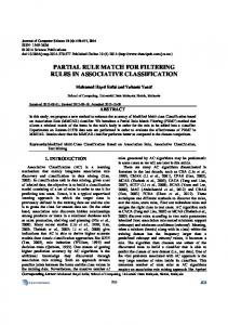
Sensitivity and specificity are thus properties of a classifier, and an ROC curve represents these measures for a range of classifiers only differing in the threshold value τ . Sample ROC curves are shown in Figure 4.2. A straight line from (0; 0) to (1 ; 1 ) indicates only random classificatory ability.

(0,1)

Sensitivity

(1,1)

1 - Specificity Figure 4.2: Sample ROC curves. Each point on the curves corresponds to a decision threshold. The dashed curve corresponds to a classifier with no discriminatory capability.

Although classifier performance should not be compared for a fixed τ , ROC curves can also be used to select a particular threshold value for a given application. Generally, the point closest to (0; 1) is a good choice if the two types of error have the same associated cost.

4.5.1 The Area Under the ROC Curve Comparing accuracy measures for different classifiers measured on the same data is relatively easily, since the accuracy values are real numbers between 0 and 1. Comparing ROC curves, however, is more difficult. If the graph for one ROC curve is greater than the graph for another (the first curve lies entirely above the second),


28

then the first ROC curve is said to dominate the second. A classifier with a dominating ROC curve are always said to be better. Generally, however, ROC curves are not dominating or dominated, but intersects at one or more points. To compare the estimated performance of classifiers with general ROC curves measured on the same data, a single-valued measure representing some of the information in the ROC curve is needed. The area under the ROC curve (AUC) is generally accepted as the preferred single number measure. In the following, the AUC for a ROC curve computed for a rule-based classifier RUL relative to a decision system will be denoted

A

AUCA ( RUL)

(4.4)

A ROC graph consists of a finite number of points, and the AUC is generally computed using the trapezoidal rule of integration. Hanley & McNeil (1982) provide expressions for approximating the standard error se( AUC ) corresponding to the computation of an AUC estimate AUC using the trapezoid rule.

4.5.2 Comparing AUC Given two classifiers, ROC analysis of the classifications of a data set (a testing set or a hold-out set) can be performed in order to compute the respective measures of performance, the AUCs, for the classifiers. Collapsing the ROC curves into single numbers allows the performance of the two classifiers to be compared. But can one be certain that one classifier is better than another if the AUC is higher? Clearly, small differences in the computed AUCs can be random. To assess whether the differences between the AUCs computed from the same data set is random or real, statistical hypothesis testing can be employed. Hanley & McNeil (1983) defines the following test statistic: Z=

AUC1 AUC2 se( AUC1 AUC2 )

(4.5)

where AUC1 and AUC2 are the AUC measures for the two classifiers. It is inappropriate to compute the standard error of the difference between two AUC values computed from the same data directly. When computed from the same data, AUC1 and AUC2 are very likely to be correlated. In the following formula for calculating the standard error for the difference, Hanley & McNeil (1983) takes into account the correlation between the classifications made by the two classifiers:

q

se( AUC1

AUC2 ) =

se21 + se22

2rse21 se22

(4.6)

where se1 and se2 are the standard errors for AUC1 and AUC2 , respectively, and r is a value that represents the correlation between the two areas. r is a function of the average value of two intermediate correlation coefficients and of the average areas. The intermediate coefficients are the correlations between the two classifiers’ certainty values for objects with negative decision and positive decision, respectively. These coefficients can be computed using either the Pearson product-moment correlation method or the Kendall tau. For a tabulation of r, we refer to Hanley & McNeil (1983). Z (Equation 4.5) is standard normally distributed under the hypothesis that the two areas really are equal, and can be used to test – under a certain significance level – whether the two areas are statistically likely to be different. For convenience we will in the following discuss the one-tailed case, where the problem is

4.5. ROC ANALYSIS

29

to conclude whether one particular classifier is better than the other or not (rather than that one of the classifiers is better than the other as in the two-tailed case). The following discussion is easily applied to the two-tailed case. Consider that AUC values has been calculated for two classifiers on the same data, and that the value of the first classifier, AUC1 , is slightly larger than the value for the second classifier, AUC2 . The one-tailed case is used to determine whether the difference is random or real. The hypotheses for a one-tailed test are: H0 : The areas are really equal, and Z is normally distributed H1 : The area for the first classifier is larger than the area for the second classifier, and Z is not normally distributed.

(4.7) (4.8) (4.9)

The hypothesis testing is done by selecting a significance level α and calculating a value, called the critical ratio, z of Z. The probability of a large absolute value z under the hypothesis that Z is standard normally distributed is low, and the null hypothesis H0 should be rejected in favor of the alternative hypothesis H1 in that case. More specifically, the null hypothesis should be rejected in the case that the p-value corresponding to the value z is lower than α or, equivalently, that the value z is higher than the Z-value zα corresponding to the probability α . These concepts are illustrated in Figure 4.3.

6

A1

0 Z

z1

A2 zα

A3 z2

Figure 4.3: Two-tailed hypothesis testing. p z2 = A3 , α = A2 + A3 and p z1 = A1 + A2 + A3 . z1 and z2 are calculated values of the test statistic Z. p z1 > α (z1 < zα ) and the null hypothesis is not rejected, leading to the conclusion that the two areas used to calculate z1 are not significantly different. p z2 < α (z2 > zα ) and the null hypothesis is rejected, leading to the conclusion that the two areas used to calculate z2 are statistically significant different.

The significance level α is the probability that we conclude that the difference is statistically significant, when it really is not (the probability that H0 is rejected when it reflects the true state of nature); see Figure 4.3:

α = Prob( Z

zα j H0 )

(4.10)

30


The lower the value of α , the more certain we can be that the difference really is significant when we conclude that it is. Testing for Statistically Insignificant Difference The hypothesis test discussed above is designed to determine, under a certain significance level, whether one classifier can be considered to perform – statistically speaking – better than another. The validity of the claim of significant difference depends on the value α ; the smaller α the more we can rely on the claim. Sometimes, however, it is the opposite conclusion that is interesting – namely whether one classifier can be considered to perform – statistically speaking – not any worse than another, that is, to have equal or better performance. Ideally, this problem could be attacked by exchanging the hypotheses H0 and H1 above and to use a test statistic with known distribution under H1 (that the significance is different). Then, one could make the claim that the two classifiers are (at least) equally good (statistically speaking) accompanied by a certain significance level. Alas, there is no such test statistic available. Lacking a proper statistic for this “direction” of the test, Equation 4.5 will be used for this purpose in later experiments. It is very important to point out what the test described above enables us to conclude regarding the “equality” between classifiers. The case of not rejecting H0 tells only that not enough evidence to support H1 was available; it says nothing statistically about the validity of H0 . In other words, saying that H0 is valid on the grounds that it is not rejected is a statistically invalid conclusion. It is natural, however, to assume that the classifiers are equal because there is not enough evidence available to conclude that they are significantly different. The difference between drawing a statistical conclusion and assuming that the null hypothesis holds because the alternative hypothesis can not be accepted is crucial. Note that if the alternative hypothesis had specified an alternative distribution for Z (instead of “not normally”), the type II error – the probability of accepting the null hypothesis given that the alternative hypothesis is true – could be calculated to accompany the assumption of equality. To summarize; when given the task of determine whether the difference between two computed values AUC1 and AUC2 (where AUC1 > AUC2 ) is statistically insignificant (that the classifier corresponding to the second value is (at least) as good as the classifier corresponding to the first value), the hypothesis test with the test statistic Z and the hypotheses H0 and H1 described above will be employed. If H0 is rejected under a small significance level, it is fairly certain that the difference is significant and we cannot conclude that the classifiers are equal. If H0 is not rejected, we can only assume that H0 is true and concludes that the difference is insignificant.

CHAPTER

5

Genetic Algorithms Often, optimization problems are search problems with very large search spaces. Genetic algorithms is a technique for finding near-optimal solutions for such problems. The first section of this chapter introduces optimization problems, while the rest of the chapter presents some aspects of genetic algorithms. See e.g. Goldberg (1989), Mitchell (1996), or Michalewicz (1996) for more comprehensive introductions.

5.1 Search as an Optimization Problem All problems can be (re)formulated as search problems. The relevant aspects of the world at a given instance of time can be captured as the state of the world at that instance and a given problem can be solved by finding a path from the initial state representing the world as it is at the time before the problem is solved to a goal state representing a world where the problem is solved, using a set of operators. The set of operators (or the successor function) assign the directly reachable states to each state. Thus, a problem can be seen as a search through a (possibly infinite) state space S = s0 ; s1 ; : : : ; sk ; : : : . Problems are often solved using additional information about the relative costs of the states and/or of the use of the different operators.

f

g

General search problems consists of finding the path from the initial state to the goal state, and a search algorithm is then a function mapping the problem – consisting of the state space with an initial state, a description of the goal states, a set of operators and possibly additional information – to a sequence of operator applications. Russell & Norvig (1995) view the operators as the actions available to an agent, and the solution to a problem is then the actions that must be performed in order to solve the problem. A search strategy is used to select the next operator to use in any given state. Uninformed search methods use strategies that are independent of the relative “goodness” of the states, examples are depth-first and breadth-first search. Such methods have poor performance – i.e. a great number of states must be visited before the goal state – for problems with large state spaces. In fact, these methods only enumerate the set of reachable states and visit them in order. Informed search methods, on the other hand, guide the search by using heuristics to evaluate the advantage of going to a particular state. Some problems specify concrete goodness measures for each state in the state

C H A P T E R 5. GENETIC ALGORITHMS

32

space. This measure is not a heuristic, which is a “qualified guess” in the lack of a proper measure, but an actual evaluation of how useful a state is as a solution. A goodness measure is an evaluation function f : f :S

!R

The goal states for problems specifying a goodness measure are implicitly defined through the goodness measure and a threshold value specifying how “good” a solution must be to qualify as a goal state. In addition, goal state is itself often a solution to the problem, and the path is not relevant. Such problems – specifying an evaluation function f and where a goal state itself is a complete solution – are optimization problems. The states that optimizes the evaluation function are sought. Since the path used to reach a state is irrelevant, so is the operators used. In an optimization problem, all states are in principle reachable from all states. Algorithms use operators to solve such problems, however, to guide the search. The difference compared to general search problems is that in the latter case operators are often a part of the problem, while for optimization problems the operators are specified by a particular algorithm. An algorithm that solves1 optimization problems is shown in Figure 5.1. G ENERIC function G ENERIC -O PTIMIZATION(S, f ) returns s inputs: S, a state space f :S R, an evaluation function

2S

!

2

find the s S that maximizes f (s) return s end function Figure 5.1: A skeleton of an algorithm that solves optimization problems

O PTIMIZATION depends only upon the given state space and the evaluation function, and returns a single state. Implementations of algorithms that solve optimization problems differ in the operators they use to move from state to state. Optimization problems can be attacked by iterative improvement methods. These methods iteratively evaluate the current state, and select an operator to increase (not necessarily in the short run) the goodness measure. Consider the state space laid out in a two dimensional coordinate system, each coordinate corresponding to a state and each neighboring coordinate corresponding to a state reachable with an algorithm operator. Now let the goodness measure correspond to a third dimension. Then the state space can be seen as a landscape with the height at each point corresponding to the goodness measure of the state at that point.Iterative improvement methods try to find the highest peaks in the landscape. Each point in the landscape is a possible solution, and the methods try to iteratively improve the quality of the current (possible) solution. Since most of these methods usually only keep track of the current state and not a list of the already visited states and in addition do not look further ahead than the neighboring states, “this resembles trying to find the top of Mount Everest in a thick fog while suffering from amnesia” (Russell & Norvig 1995, p. 111). Nevertheless, traditional iterative improvement methods like hillclimbing and simulated annealing perform well on certain kinds 1 An algorithm can seldom be sure that there does not exist a better solution (without traversing the complete search space). The term “optimization” is thus abuse of language, but is very commonly used in the literature.

5.2. INFORMAL INTRODUCTION TO GENETIC ALGORITHMS

33

of problems. These methods are briefly introduced below. Genetic algorithms is another method that can be said to use an iterative improvement technique, although it has little in common to the other methods mentioned. This method is inspired by biological evolution, and iteratively updates a “population” of possible solutions by replacing the members of the population with new possible solutions that inherit properties from the best members of the old population.

5.1.1 Iterative Improvement Algorithms Hillclimbing Hillclimbing techniques always select the state that improves the goodness of the current state the most as the next state. That is, they always move in the direction of the steepest upward slope2 . Obviously, these algorithms are not good for solving optimization problems in general. The most important drawback is that the algorithms halt if they find local maxima3 , that is, peaks that are lower than the highest peak. The success of a hillclimbing algorithm is thus highly dependent upon the starting point. A hillclimbing technique that tries to remedy this problem is iterative, or random restart, hillclimbing. This technique tries to find global maxima by running multiple iterations with different starting points.

Simulated Annealing Instead of always moving up the steepest slope, simulated annealing techniques includes the possibility of taking a step downward to escape local maxima. When the algorithm reaches a peak, it can move to a lower state with a probability exponentially inversely proportional to the difference between the goodness of this state and of the current state. This probability is also positively dependent of the “temperature” of the system. As the temperature is gradually lowered, fewer and fewer changes are being made, until the algorithm terminates (at which point the temperature is zero and the algorithm behaves like a hillclimbing algorithm).

5.2 Informal Introduction to Genetic Algorithms Algorithms loosely based on simulated evolution are often referred to as evolution programs (EPs). An EP maintains a population of individuals, each individual representing a possible solution to a problem. Each individual has an associated fitness. The population is updated by generating a new generation of individuals on the basis of the current generation. The principles of evolution are used to create the new generation. For instance, parent individuals are selected stochastically according principle of natural selection (survival of the fittest), to be combined to create offspring individuals. Offspring individuals inherit the parents’ features (or genes). Another mechanism inspired by nature is mutation of single features – removal or addition of single genes. The mechanisms that are used to create new individuals from old individuals are called genetic operators. 2 If the evaluation function is a cost function rather than a goodness function, these techniques are called gradient descent techniques and move in the direction of the steepest downward slope. 3 Or local minima, in the case of gradient descent techniques.


34

Examples of natural selection in nature are plenty: an individual with “bad” genes (e.g. a bird with a very different color than that of the tree it lives in) has a higher probability of not surviving in its environment (e.g. being spotted by a predator). Thus, the probability that individuals with “good” genes will reproduce is higher than that of the individuals with “bad” genes, and the “good” genes (or good combinations of genes) have a higher chance of being carried on to the next generation (an example is a whole population of birds changing color over a number of generations). This mechanism is the motivation behind the use of EPs. By selecting the best individuals for reproduction, it is hoped that good combinations of genes will be found and that the average fitness of the population increases4 . Michalewicz (1996) defines as EPs all algorithms that are based on the principles of evolution and that maintains some kind of population, without any restriction on the representation of the individuals. Generally, EP individuals may have any representation, e.g. a tree, a DAG, a bitstring or a planning schedule. In the evolutionary programming literature the term genetic algorithm (GA) tends to be reserved for algorithms that represent individuals as fixed-length binary bitstrings. Michalewicz (1996, p. 3) defines (classical) GAs as:

Using fixed-length binary bitstrings Using only the two binary genetic operators crossover and mutation

In this thesis the term genetic algorithm will denote an EP with fixed-length bitstring representation that only uses general evolution-inspired genetic operators (not necessarily limited to crossover and mutation). The more general class of EPs contain algorithms with problem-specific genetic operators. The main difference between a general EP and a GA is that to solve a problem using a EP, an algorithm attacking the particular problem is generally constructed, while to solve a problem using a GA, the problem must be reformulated to fit into a standard GA algorithm. Genetic algorithms are commonly employed to solve optimization problems (see the previous section). They are massively parallel iterative improvement methods, where small genetic changes are performed on the the best individuals (i.e. states) in order to breed better individuals (move up the hill). The parallelism and the indeterminacy introduced by the common genetic operators ensures that the algorithm does not get stuck on local maxima.

5.3 Genetic Algorithms Defined 5.3.1 Concepts Formal definitions of GA concepts are uncommon in the literature. In this section, general definitions of some concepts – as they will be used in this thesis – are presented. As a common terminology does not exist, the definitions of the following concepts are not necessarily shared by other authors. The most important concept in a GA is the individual, which consists of a set of i m 1) is a member of a finite genes. A gene, or a feature or a decoder, g i (0 set G = g 0 ; g 1 ; : : : ; g m 1 .

f

g

4 EPs ignores the experiences (the relation between actions and rewards) learned by an individual in its lifetime; the evolution model is not Lamarckian.

5.3. GENETIC ALGORITHMS DEFINED

35

Definition 5.1 (Individual, Chromosome Space). Given a set of genes G, the chromosome space over G is UG = P( G ). A member I UG is called an individual, or a chromosome.

2

In classical GAs (Holland 1975), individuals are represented by strings of bits, where each “1” (“0”) indicates the presence (absence) of the particular gene in the individual corresponding to the position of the bit5 . The string positions are called loci. Definition 5.2 (String). Given a set of genes G, a string, or bitstring, B over UG bj Gj 1 where bi 0; 1 (0 i G 1 ). is a sequence B = b0 b1

2f g j j

Definition 5.3 (Semantics of a String). Given a set of genes G, the semantics of a string B = b0 b1 bj Gj 1 over UG is the individual I = [ B℄ UG :

2

[b 0 b 1

b j Gj

1℄ =

f g i jbi = 1 g

The [℄ operator is isomorphic to a bijective function, and the corresponding inverse is denoted [℄ 1 ; e.g. B = [ I ℄ 1 .

Given a set of genes G, a bitstring B over UG thus uniquely identifies an individual I UG . We will often refer to individuals by their corresponding bitstring, and sometimes – by abuse of language – talk about the individual B.

2

As mentioned in section 5.1, optimization problems use a goodness measure that operates on the states in the state space. In GAs, the goodness measure is called a fitness function. Definition 5.4 (Fitness Function). A fitness function on a chromosome space UG is a function: f itness : UG

!R

GAs operate on collections of individuals called populations. Definition 5.5 (Population). A population P over a chromosome space UG is a set of individuals P

UG

A population is evolved into a new population by applying genetic operators to the members of the population. Definition 5.6 (Genetic Operator). A genetic operator f of order k over a chromosome space UG is a function f : (U G ) k

! (U G ) k

5 In

this chromosome model, each gene can be in one out of two states; “on” (present) or “off” (absent). In natural genetics, a gene can have more than two possible states called alleles or feature values.


36

The procedure used to apply a genetic operator to a set of individuals in a population is called a genetic operation. A genetic operation samples a set of parents and selects the particular genetic operators to be used from a class of operators. The two standard GA operators are mutation and crossover. Definition 5.7 (Mutation). The first order genetic operator m p : UG where m p ([b 0

where 0

p jGj

b p b j Gj

b¯p

;

b j Gj

UG

1℄

The second order genetic operator x M : UG UG !

1, is a mutation operator over UG .

Definition 5.8 (Crossover). UG UG where

x M ( [ B1 ℄ ; [ B2 ℄ ) = ( [ B1

2

1 ℄) = [b 0

!

M + B2 M¯ ℄ [B1 M¯ + B2 M℄) ;

for some M [UG ℄ 1 , is a crossover operator over UG . M is called the crossover mask, and for Ia ; Ib UG , the individuals in the pair f ( Ia ; Ib ) are called offspring.

2

(In the preceding definitions, B¯ denotes the binary inverse of a (possibly singular) bitstring B, and and + the bitwise binary operations and and or, respectively). If the crossover mask is a continuous sequence of “1”s followed by a continuous sequence of “0”s, the operator is a single point crossover operator. Similarly, an operator with a mask consisting of a “1”s followed by “0”s and ending in a sequence of “1”s is a two-point crossover operator, and so on.

Application of these two types of genetic operators is illustrated by the next pair of examples. Example 5.1 Consider the mutation operator m3 applied to the individual I1 = [11010011℄ The result of the application is the individual m3 ( I1 ) = [11000011℄

Example 5.2 Consider the single point crossover operator x 11111000 applied to the individuals I2 = [1011100℄ I3 = [00100110℄ The result of the application is the pair of individuals I4 and I5 : [ I5 ℄ =

[ I2 ℄ =

j

!!

z}|{

10111 | {z } 000

aaa

a! !!! aaa

aa z }| {

[ I3 ℄ =

aaa

[ I4 ℄ =

j

j

00100 000 | {z } |{z}

z }| { z}|{

j

j

00100 |{z} 110

!! ! ! !!

10111 110

where the bar ( ) in the bitstrings denotes the single crossover point.

5.3. GENETIC ALGORITHMS DEFINED

37

5.3.2 A Genetic Algorithm An example of a generic genetic algorithm is shown in Figure 5.2. function G ENETIC -A LGORITHM(G, f itness, I NIT(g), S TOP(stats), R E SAMPLE (p), PARENT S ELECT(p), U PDATESTATS(p,f), R ECOMBINATE(p,o), G ENETIC O PERATION 1 (p), : : : , G ENETIC O PERATION j (p)) returns Stats, statistics inputs: G, a set of genes R, a fitness function f itness : UG I NIT(g), a function returning a population UG S TOP(stats), a stopping criteria R ESAMPLE(p), a function sampling a new population from an old PARENT S ELECT(p), a parent selection function U PDATESTATS(p,f), a function updating statistics from a population and a set of fitness values j), functions implementing genetic operG ENETIC O PERATION i (p) (1 i ations R ECOMBINATE(p,o), a function recombining offspring with a population

!

P I NIT(G) for all Ii P do Fi f itness( Ii ) end for Stats U PDATESTATS(P,F) while not S TOP(Stats) do R ESAMPLE(P) P PPar PARENT S ELECT(P) for i := 1 to j do G ENETIC O PERATION i ( PPar) O f f spring end for P R ECOMBINE(P,O f f spring) end while return Stats end function

2

Figure 5.2: A genetic algorithm

Implementations of GAs differ with respect to the input parameters to G ENETIC A LGORITHM. I NIT generates the initial population. The algorithm updates statistics such as average and maximum fitness in each iteration, and it’s termination is determined by S TOP. A new generation is generated from an old one by the R ESAMPLE function which resamples the population. The resampling is generally done from a distribution that represents the fitness distribution of the individuals.

j) implement the genetic operations The functions G ENETIC O PERATION i (1 i which sample from the parent population created by the function PARENT S ELEC TION. An individual in the parent population is selected by the genetic operation G ENETIC O PERATION i with probability p i . Let size be the size of the population. A genetic operation:

1. Samples p i size k-tuples from the parent population


38

2. For each k-tuple; selects a genetic operator from a predefined set of genetic operators of order k and applies it to the tuple 3. Returns the set of offspring from the genetic operations The selection of a genetic operator of a predefined type, e.g. two-point crossover operators (which corresponds to selection of the crossover points), is generally done randomly. The final recombination of the offspring into the population is done by the function R ECOMBINATE, for example by replacing the parents with the offspring.

5.4 Genetic Algorithms and Optimization Problems Genetic algorithms are often used to solve optimization problems. Such problems consist of a state space S and a goodness function f , see figure 5.1. To use a GA to solve an optimization problem, the user must create a coding of the state space by constructing the following structures:

G, the set of genes used to span out the chromosome space meaning : UG state space

! S, a function used to map an individual into a state in the

Clearly, UG is the GA’s representation of S. The meaning of an individual, its phenotype, is of no concern to the GA. An algorithm solving a problem using a GA uses the function meaning to map from, for example, the best individual found by the GA to a (goal) state. The selection of a gene set G is arbitrary as long as the cardinality is large enough to represent S (2 j Gj S ). In some problems, however, the states can be decomposed into genes in a very natural way. Figure 5.3 shows an algorithm that solves optimization problems using a GA. The function G ET-

j j

function G ENETIC -O PTIMIZATION(S, f , G, meaning) returns s inputs: S, a set of states R, a goodness function f :S G, a set of genes meaning : UG S, a mapping from individuals to states

2S

!

!

G ET G ENETIC PARAMETERS() Parameters I F IND B EST I NDIVIDUAL(G ENETIC -A LGORITHM(G, Parameters)) return meaning( I ) end function

f

Æ

meaning,

Figure 5.3: Solving an optimization problem using a genetic algorithm

G ENETIC PARAMETERS() retrieves all but the three first parameters to G ENETIC A LGORITHM( : : : ). F IND B EST I NDIVIDUAL(stats) returns the best individual computed by the GA from a statistic structure. The fitness function used by the genetic algorithm maps an individual I into a real number r through the composition of the goodness function and the meaning function: I

2 UG meaning 7! s 2 S 7!f r 2 R

(5.1)

5.5. THEORETICAL FOUNDATIONS where s

39

2 S.

5.5 Theoretical Foundations Although a solid theoretical basis for genetic algorithms is lacking, some results exist and are commonly referenced in the literature. The aim of these results is to explain why GAs work, i.e. why they can be used to find iteratively better solutions. Hypotheses trying to explain why GAs work often use the notion of a schema. Schemata are strings over the bitstring alphabet augmented with the “don’t-care” character “*”. A schema denotes the subset of the chromosome space (the solution space) containing all the individuals represented by bitstrings that matches the schema in all non-”*” positions. Schemata make it possible to talk about similarities of groups of individuals. Definition 5.9 (Schema). Given a set of genes G, a schema S over G is a sesj Gj 1 where si 0; 1; (0 i G 1). The order of a quence S = s0 s1 schema is

2f

o( S) =

g j j

jfsi jsi 6= gj

The defining length of a schema is

δ ( S) = j i where i ( j) is the smallest (largest) number such that si 6= (s j 6= )

Definition 5.10 (Semantics of a Schema). Given a set of genes G, the semantics of a schema S = s0 s1 sj Gj 1 is the set of individuals I0 ; : : : ; Ik = [ S℄ UG :

[ S℄ =

f

g

f [ B0 ℄

;::: ;

[ Bk ℄

f

g

g

where B0 ; : : : ; Bk is the largest set of bitstrings such that, for all B j = b j0 and all i (0 i G 1),

j j

, bj si = 1 , b j si = 0

i

=

0

i

=

1

b j Gj j

Consider the schema S = *0*101**. S represents a set of individuals containing e.g. 00010100 and 10010101 ([00010100℄; [10010101℄ [*0*101**℄). The order of the schema is the number of non-”*” characters, o( S) = 4. The defining length is the difference in position between the last and the first non-”*” character in the schema, δ ( S) = 4.

2

\

The set of individuals in a population P matched by a schema S is P [ S℄. The average fitness of a schema S in a population P is the average fitness of the individuals in P matched by S. Under certain conditions, it can be concluded – by careful analysis of the number of individuals in a population matched by a schema S at a given time for “good” schemata S (see e.g. Michalewicz (1996)) – that the sampling rate of an above average schema increases with the number of iterations. This conclusion is called the Schema Theorem, or the Fundamental Theorem of Genetic Algorithms.

1

40

C H A P T E R 5. GENETIC ALGORITHMS Hypothesis 4 (Schema Theorem) Schemata of small defining length, low order and above-average fitness receive exponentially increasing trials in subsequent generations of a genetic algorithm.

Thus, the more fit schemata will grow in influence in a population, especially if the non-”*” characters are few and close together. Such schemata are called building blocks. The following hypothesis is often claimed to be valid. Hypothesis 5 (Building Block Hypothesis) A genetic algorithm seeks near-optimal performance through the juxtaposition of short, low-order, high-performance schemata, called the building blocks.

The building block hypothesis describes the workings of the GA machinery like “a child [that] creates magnificent fortresses through the arrangement of simple blocks of wood” (Goldberg 1989, p. 41), and it has shown to hold on a wide range of empirical studies. The hypothesis is, however, highly controversial in the GA community. It builds on empirical studies rather than on formal proofs, and constructing examples that violates the hypothesis is not very difficult. Although widely cited, also the schema theorem fails to provide a proper theory of the workings of genetic algorithms in general. Thus, lacking a theoretical foundation, Hypotheses 4 and 5 should be used as explanations of why GAs often work in practice, rather than as proofs of formal properties.

Part II

Rule Filtering

CHAPTER

6

Rule Filtering Hypothesis 1 (on page 3) states that a given complex model can be replaced with a model of a descriptive nature without lowering the predictive performance significantly. One strategy for finding a simple model with good classificatory capabilities is first inducing a general – possibly complex – model, and then pruning this model in a way that does not lower the performance significantly. Pruning can be done by identifying and removing the components of the model that only explain small parts of the data – e.g. random noise – thereby preserving the general trends in the underlying data material. In this chapter one particular method for pruning rule based models, called rule filtering, is introduced. Two concrete algorithms for rule filtering are then presented in the two following chapters. Empirical experiments employing these algorithms are documented in the last part of the thesis.

6.1 Model Pruning In Chapter 1, the following properties of descriptive models were identified: 1. They are not too complex to be comprehended by humans 2. They exhibit acceptable performance, compared to more complex models Here, model pruning is used to find such models. Model pruning involves postpruning (see Section 1.3.1) an already induced model, in contrast to using prepruning techniques to create small models in the inductive learning step. Model pruning can thus be seen as an independent step used after the induction step in the knowledge discovery process, and can be used on any model regardless of the concrete algorithm used to induce the model.

M

Let MOD be a set of possible models for a phenomenon, and let the relation be a partial ordering on MOD. (MOD; ) denotes a partial ordered set (poset). A 0 in (MOD; ) is called a submodel of a model 0 model in (MOD; ) if . In model pruning, submodels satisfying the two properties stated above are sought. To this end, two corresponding functions must be defined on the set of models. A performance function is used to compare the performance of the models:

M

M

performance : MOD

M

! [0

;

1℄

C H A P T E R 6. RULE FILTERING

44

All performance functions discussed here are assumed to be normalized to the with performance measure performance( ) = 1 is a interval [0; 1℄. A model perfect model for the phenomenon1 . A complexity function is used to compare the complexity of the models:

M

M

complexity : MOD

!R

+

The following is assumed to hold for a complexity function:

M2 M1 ) complexity(M2 ) complexity(M1 ) M

M

(6.1)

complexity( ) is a measure of the complexity of the model . We will be con0 cerned with the relative complexity – the degree of complexity of a submodel compared to the model . The relative complexity is given by a function complexityM : MOD [ 0 ; 1 ℄:

M

!

M

complexityM (

(M ) M0 ) = complexity complexity(M)

0

M

(6.2)

Clearly, model pruning is an optimization problem (see Section 5.1) with state in (MOD; ), model pruning involves the space S = MOD. Given a model following steps:

M

1. Defining the complexity and performance functions 2. Defining the evaluation function f : MOD ity and the performance

! R as a function of the complex-

3. Solving the optimization problem defined by MOD and f by traversing the 0 0 0 maximizing f ( 0 ). to find the submodel search space

fM jM Mg

M

M

6.2 Rule Filtering The models under consideration in this thesis are sets of propositional decision rules (Chapter 3). How such sets can be used as classifiers was discussed in Section 3.6. Rule filtering operates on an existing (potentially large) model, pruning it while retaining performance. Since the motivation for finding smaller models is that the models generated by the induction algorithms consist of a large number of rules (see Section 1.3), we suspect that individual rules can be removed from the large rule sets without lowering the performance of the resulting classifiers. Rule filtering attempts to find good submodels by removing whole rules. In model pruning using rule filtering, the set of possible models, given a rule set RUL, is the power set of RUL: MOD = P(RUL). Submodels are defined as subsets, the submodel relation equals the set inclusion relation .

1 It may be the case that a perfect model does not exist, for example when the available information is insufficient to create a model with the desired resolution, or when the data collection procedure has been subjected to noise.

6.3. EVALUATING SUBMODELS

45

6.2.1 Complexity The complexity of a rule based model RUL can be defined in several ways. Two of them are: complexitycard (RUL) = RUL

j

j

(6.3)

complexitydescr (RUL) =

number of descriptors in r

(6.4)

∑

2

r RUL

Both functions define complexity to be proportional to the number of “atomic” constituents in a model. They differ in regards to the resolution; in equation 6.3, single rules are considered to be the basic elements, in contrast to single descriptors in equation 6.4. The latter is the traditional measure of complexity of boolean formulae – complexity being equal to the number of boolean connectives (Pearl 1978) – over the language of decision rules. Another, more general, possibility is to associate costs to the individual attributes in , and let the complexity function be a function of the costs of the attributes in the rules’ antecedents. This scheme is useful in domains where values for some attributes are more difficult or expensive to obtain than for others. Examples are results from different types of medical tests.

A

6.2.2 Performance Methods for measuring the performance of classifiers were presented and discussed in Chapter 4. These methods measure the performance relative to a decision system. See Section 6.5 for some comments regarding optimizing the performance on a particular data set. Both the accuracy and the area under the ROC curve can be used as performance measures for rule filtering.

6.3 Evaluating Submodels Based on the discussion in Chapter 4, we find that the area under the ROC curve is the proper measure for comparing classifier performance. AUCA will henceforth be used as the performance measure relative to a decision system . In the following, it will be assumed that the decision system and the ROC focus class used in calculating the AUC is implicitly given. In an application of rule filtering, these will be set by the user.

A

A

Selecting a complexity function is not easy. The rule filtering process contains many other degrees of freedom, and the current investigation must be limited to one complexity function only. To this end, we have chosen to use the rule set cardinality as a measure of complexity instead of the more traditional complexity measure. The main reason for this is the idea for a strategy for limiting the search space of submodels if a “quality measure” can be defined on the level of the individual atomic constituents of a model. Several such quality measures are defined for individual rules. Further rationale is the experience that long rules in an induced rule set most often are due to noise in the originating decision system, and thus have low support counts. Therefore, long rules contributes little to the overall performance of a rule set, and will seldom be selected for inclusion in a filtered model if equation 6.3 is used. Using the rule count to evaluate complexity will thus not, in the general case, lead to models with high descriptor counts.

C H A P T E R 6. RULE FILTERING

46

f

fr 1

;::: ;

rn

f

f

g

RUL = r1 ; : : : ; rn SSS SSS jjjj j j SSS j j SS jjjj 1

g

fr 2

f

f g

rn

g

g

r1 ; r2 ; r3 TTTT nn TTTT n n n TTTT n n n T n r1; r2 r1 ; r3 T r ;r PPP j 2 3 TTTT PnPnPnnn TjTjTjTjjjj TTTT nn PPPP jjj TT nnn jjjj r1 r2 r3

g

;::: ;

g

f g

f

g

f g

Figure 6.1: Hasse diagram of the lattice ( P (RUL);

).

The role of the evaluation function is to weight between the complexity and the acceptable performance of a submodel. The choice of a function combining the complexity and performance measures is user, application and domain dependent. In one application, for example, only models with five or fewer rules are interesting, no matter how good performance larger models might have. In another application, the evaluation criterion might be that the performance should be no lower than 99% of the performance of the unfiltered rule set, even if there exists considerably smaller models with performance equal to 98% of that of the unfiltered set. In the next chapters, two algorithms for finding good, small submodels are presented. The choice of the form of the evaluation function is discussed in connection with one of these algorithms. In the other algorithm, the evaluation criterion is implicitly defined in the algorithm itself, and needs no explicit definition.

6.4 Searching Having defined an evaluation function over the submodels, model pruning is performed by searching the space of submodels for the best model according to the function. The cardinality of the search space for rule based models is:

j Sj = jfRUL0 jRUL0 RULgj = 2jRULj (6.5) Clearly, the poset ( P(RUL) ) is a lattice2 . The search consists of traversing the lattice. The evaluation function can be tweaked to determine the optimal point(s) in the lattice. An outline of the submodel lattice for a rule set RUL = fr1 rn g ;

;::: ;

is shown in Figure 6.1. Each node in the diagram can be seen as being labeled with a complexity measure and a performance measure, and the node chosen by the search algorithm is determined by the evaluation function.

Typical induced rule sets, such as those computed by the R OSETTA system (Øhrn et al. 1998a), can have cardinalities with magnitudes of 100,000 rules. Clearly, the search space corresponding to such models are too large to be traversed by conventional search strategies, and other methods must be used. 2 The least upper bound and greatest upper bound of two elements A and B of ( P (RUL) ; and A B, respectively.

\

) is A [ B

6.5. COMMENTS

47

6.5 Comments The rule filtering problem was described as an optimization problem because the performance of the pruned models could be assessed. The problem is that a performance measure is accurate only for the data set used to compute it. The assessed performance tells only to what degree a theory fits the part of an equivalence relation represented by the data set, it can tell us nothing about how well the theory fits the complete goal relation. This problem is really implicit in inductive learning. Inductive learning is like telling the future; if we have access to an oracle that can verify the performance of the crystal ball, we do not need the crystal ball because we can use the oracle in the first place. Likewise, to assign a correct performance measure to a theory we would need access to the correct partition, and if we have access to the correct partition we need not construct the theory. Therefore, the assessed performance can never be more than an estimate. The question then is whether this estimate is good enough to be used to compare models, that is, if it should be used to define rule filtering as an optimization problem. Ideally, statistical tools should be used to give a better answer to whether the difference in estimated performance between two models are statistically significant. Unfortunately, the computational complexity and practical running times of the algorithms presented in the next chapters prevent anything but straightforward comparisons. It must be kept in mind that defining rule filtering as an optimization problem is a simplification, and that the algorithms actually only optimizes the performance on a hold-out set. If both the hold-out set and the testing set represent the “real” distribution of data in the particular domain, the models with high estimated performance on the hold-out set will also have high estimated performance on the testing set.

CHAPTER

7

Quality-Based Filtering 7.1 Introduction Generally, the cardinality of the search space corresponding to the rule filtering optimization problem is extremely large. One solution to this problem is employing special search algorithms, such as genetic algorithms. This possibility is explored in the next chapter. In this chapter, an algorithm that only explores a very small, well-defined fraction of the search space is investigated. The motivation was stated in Hypotheses 2 and 3 on page 4. Hypothesis 2 states that there exist a function creating an ordering of the rules in a rule set, such that a minimal model satisfying a given performance constraint can be obtained by successively including the rules with the best quality measures until the constraint is satisfied. A great number of small models (subsets of a rule set) generally exists. Hypothesis 3 on page 4 states that the models consisting of the “best” individual rules in the ordering also are the overall best models. The function creating the ordering of the rules will be called a quality function, and will be defined as assigning a “quality” measure to each rule. Rule quality is, in addition to overall model performance, another evaluation measure, but on the level of single rules instead of sets of rules. The hypothesis effectively states that the performance of a model is a function of the performance (quality) of the single rules. According to this hypothesis, for a given model performance constraint, the best submodel is unambiguously defined by iteratively increasing the threshold and removing rules until no more rules can be removed without violating the model performance constraint. If Hypothesis 3 holds, the rule filtering problem can be easily solved since only at most one model of a given complexity needs to be considered. In the following section, several formulas for measuring quality are presented.

7.2 Defining Rule Quality The rule quality for the rules in a rule set RUL is determined by a quality function: quality : RUL

!R

(7.1)

Defining a quality function consists of identifying the properties of “good” rules. The function is defined so that is maximized for certain properties. Two properties commonly used to define “good” rules is accuracy and coverage (see Definitions 3.7

C H A P T E R 7. QUALITY-BASED FILTERING

50

and 3.8 on page 20). The first property is a measure of how reliable – or accurate – a rule is, the second is a measure of how important – or powerful – a rule is. Generally, we would like rules to be both accurate and powerful. The question is how these two measures should be combined to one numerical overall quality measure. The literature is rich with functions combining the accuracy and coverage properties, as well as other properties calculated from the contingency table (Section 3.4), for various purposes. Bruha (1997) summarizes some of the approaches1 . In the following, different contingency table based rule quality formulas are presented.

7.2.1 Rule Quality Formulas The formulas given below are relative to the contingency table for the given rule. U refers to the cardinality of the originating information system, i.e. the total sum in the contingency table.

j j

Michalski Michalski (1983) suggests that high accuracy and coverage are requirements of decision rules. Bergadeno et al. (1988) combine these measures into a quality measure similar to the following function:

quality Michalski(r) = µ accuracy(r) + (1

µ ) coverage(r)

(7.2)

quality Michalski is a weighted sum of the measures of the accuracy and the coverage properties; the weight µ will henceforth be called the accuracy bias. The accuracy bias is typically user defined, and is generally selected on an experimental basis. Thus, using equation 7.2 can be seen as an empirical approach without any theoretical foundation. Torgo One variation of equation 7.2, is the accuracy bias employed by Torgo (1993):

µ=

1 1 + accuracy (r) 2 4

(7.3)

In the above equation, µ is not fixed but a function of the accuracy. The formula is based on experiments by Torgo on real world domains, and the accuracy value is judged to be the most important of the two properties in equation 7.2. Brazdil Brazdil & Torgo (1990) define a quality function as a product of the accuracy and coverage measures instead of a sum:

quality Brazdil (r) = accuracy(r) ecoverage(r)

1

(7.4)

Similar to the Michalski and Torgo functions, quality Brazdil is based on empirical experiments, rather than on theoretical foundations. 1 Actually in the context of classifying

3.6.

schemes for unordered rule sets, as briefly discussed in Section

7.2. DEFINING RULE QUALITY

51

Pearson χ2 statistic Bishop et al. (1991) describe several measures related to the contingency table. Bruha (1997) has found that two of these statistics may be used as measures of rule quality. One of the statistics is the Pearson χ2 statistic: quality χ2 (r) =

nα ;β n:α ;:β nα ;:β n:α ;β nβ n:β nα n:α

(7.5)

The statistic is χ2 distributed with one degree of freedom. G2-likelihood statistic The other statistic described by Bishop et al. (1991) and recommended by Bruha (1997), also χ2 distributed with one degree of freedom, is the G2-likelihood statistic:

j j

j j

nα ;β U nα ;:β U quality G2 (r) = 2 nα ;β ln + nα ;:β ln nα nβ nα n:β

(7.6)

j j

The G2-likelihood statistic divided by 2 U is equal to the J-measure (Smyth & Goodman 1990): quality J (r) =

quality G2 (r) 2U

j j

(7.7)

Cohen Cohen (1960) presents a measure from the contingency table, interpreted as a rule quality measure by Bruha (1997): quality Cohen (r) =

jU j nα β + jU j n:α :β nα nβ jU j2 nα nβ n:α n:β ;

;

(7.8)

Equation 7.8 is measure of the sum fα ;β + f :α ;:β in the frequency based contingency table, corrected by the sum fα fβ + f :α f :β and normalized. A large value for the sum of fα ;β and f :α ;:β is clearly a desired property of a decision rule.

Coleman Bishop et al. (1991) define a measure, called the Coleman function, similar to the Cohen formula: quality Coleman(r) =

jU j nα β nα nβ nα n:β ;

(7.9)

Equation 7.9 only considers the first element fα ;β in the main diagonal, instead of both elements as in equation 7.8. The Coleman quality function exhibits high quality for a rule if many of the objects covered by the antecedent also are covered by the consequent. Unlike the Cohen function, it does not reward agreement between the number of objects not covered by the antecedent and the consequent, respectively. The Coleman function thus gives a measure of the accuracy2 , while the 2 However, accuracy (r ) fβ . 1 fβ

the Coleman function is not identical to the accuracy function; qualityColeman(r ) =


52

Cohen function also includes a measure of the coverage. Bruha (1997) proposes the two following modifications of the Coleman function to introduce coverage dependence: 2 + quality Cohen (r) 3 1 + coverage(r) quality C2 (r) = quality Coleman(r) 2 quality C1 (r) = quality Coleman(r)

(7.10) (7.11)

Kononenko The following function is an information theoretical measure of rule quality, proposed by Kononenko & Bratko (1991): quality Kononenko(r) =

log2 fβ + log 2 accuracy(r)

(7.12)

7.2.2 Discussion The Michalski, Torgo and Brazdil formulas are empirical, ad-hoc formulas, but are intuitive and interpretable. The rest of the formulas are based on theoretical foundations, and may be more difficult to interpret directly. Pearson, G2/J, Cohen and Coleman/C1/C2 are based on statistics and the theory of contingency tables. The two former formulas give association measures for the contingency table, while the two latter give agreement measures (see Bishop et al. (1991)). The Kononenko formula is based on information theory. A summary of the rule quality formulas is given in Table 7.1. The table shows the domain and range for each function. The domain for a function is considered to be all possible rules modulo some assumptions given below, except those with contingency matrices corresponding to the “Undefined when” column. The ranges are not given relative to a particular decision system. For example, the range for 1); 1℄ for a particular decision system. the Coleman formula is [ ( U

j j

Function Domains It is assumed that nα > 0 (that a rule covers at least some of the objects) and that both nβ > 0 and n:β > 0 (that there exist objects of both classes for a binary decision attribute). Rules violating the first assumption make no sense, and generating decision rules for decision systems violating the second assumption is superfluous. These assumptions are also necessary for the rule accuracy and coverage to be well-defined. An additional assumption is made regarding the association based formulas. These formulas are only valid if the class indicated by β is the dominating decision class for the rule, that is, if nα ;β > nα ;:β. The implementation of the algorithms will ensure that this assumption is not violated, see Section A.4 in the appendices. However, some of the formulas are undefined even for certain contingency matrices and decision tables not violating the above assumptions, as given by the “Undefined when” column in Table 7.1. For example, the Pearson formula is undefined when the rule covers all the objects in the decision system, and the G2 and J formulas are undefined if the rule classifies all objects correctly.

Michalski Torgo Brazdil Pearson G2 J Cohen Coleman C1 C2 Kononenko

Formula

µ accuracy(r) + (1 µ ) coverage(r) Michalski with µ = 12 + 14 accuracy (r) accuracy(r) ecoverage(r) 1 (nα ;β n:α ;:β nα ;:β n:α ;β )=(nβ n:β nα n:α ) 2 (nα ;β ln (nα ;β jU j=(nα nβ )) + nα ;:β ln(nα ;:β jU j=(nα n:β ))) quality G2 (r)=(2jU j) (jU j nα ;β + jU j n:α ;:β nα nβ )=(jU j2 nα nβ n:α n:β ) (jU j nα ;β nα nβ )=(nα n:β ) quality Coleman(r)((2 + quality Cohen (r))=3) quality Coleman(r)((1 + coverage(r))=2) log2 fβ + log 2 accuracy(r)

Range

Undefined when

[0; 1℄ [0; 1℄ [0; 1℄ [0; 1℄ [0; ℄ [0; ℄ [ 1; 1℄ [ ; 1℄ [ ; 1℄ [ ; 1℄ [ ; 0℄

1 1 1 1 1 1

n:α = 0 nα ;:β = 0 nα ;:β = 0 = nα nβ + n:α n:β

7.2. DEFINING RULE QUALITY

Quality measure

jU j 2 jU j2 = nα nβ + n:α n:β accuracy(r) fβ

Table 7.1: Summary of quality functions

53


54 Available Results

Bruha (1997) has tested the applicability of the above quality measures with different classification schemes. The investigation indicates that all the measures may be monotone towards the accuracy and coverage, but this cannot be proved for all the formulas. The experiments show that all the tested measures where applicable for the particular task, and that the empirical measures exhibit quite good performance in spite of the lack of theoretical foundations. The statistical measures were found to perform somewhat better, but no statistical significance test is used to detect any significant difference between the empirical and the statistical measures. The Michalski formula generally showed better performance with higher accuracy weights.

7.3 Quality-Based Rule Filtering Having defined a quality function quality, filtering a rule set RUL can be done by selecting a submodel RUL0

2 ffr 2 RULjquality(r) tgjt 2 Rg

As a matter of convenience, a rule set corresponding to the particular threshold value t above will be denoted RULt . Observe that the set of submodels corresponding to threshold values for a given quality function not necessarily contains a rule set with a particular cardinality RUL0 < RUL , since the quality function can map two or more rules to the same quality value.

j

j j

j

The function Q UALITY T HRESHOLD -P ERFORMANCE -G RAPH in Figure 7.1 creates a graph from a subset of R to the interval [0; 1℄, corresponding to the estimated performance of the rule set RULt as a function of the threshold value t. The minimum number of rules included for each threshold value is determined by R ESO LUTION(k), where k is the rule count for the previous threshold value. Resolution is further discussed in Section 7.3.3. The actual rule pruning can be performed by selecting a threshold, and thus the corresponding rule set RULt , from the graph. This simple algorithm is shown in Figure 7.2. Example 7.1 (Quality-Based Rule Filtering) The rule set RUL is to be filtered using the rule quality function quality. The workings of Q UALITY T HRESHOLD P ERFORMANCE -G RAPH is illustrated in Table 7.2. The table shows the rules in rk

t = quality(rk )

per f ormance( RULt )

r1 r2 r3 r4 r5

0.92 0.87 0.87 0.83 0.79

0.56 0.74 0.74 0.75 0.81

:::

:::

:::

Table 7.2: The sorted rules in Q UALITY T HRESHOLD -P ERFORMANCE G RAPH

RUL sorted by quality, and the classifier performance corresponding to the accumulated rule set. For example, RUL0:87 = r1 ; r2 ; r3 . The graph computed

f

g

7.3. QUALITY-BASED RULE FILTERING

55

function Q UALITY T HRESHOLD -P ERFORMANCE -G RAPH(RUL, R [0; 1℄ quality) returns (t; p) inputs: RUL, a set of rules [0 ; 1 ℄, a performance function per f ormance : P( RUL) quality : RUL R, a rule quality measure

f

g

per f ormance,

!

!

Sort the rules in RUL according to quality. Let the tuple (r1 ; : : : ; rj RULj ) denote the sorted rules, where quality(ri ) quality(r j ) if i j. 1 k G while k RUL do RUL0 m 0 R ESOLUTION(k) n repeat t quality(rk ) repeat RUL0 RUL0 rk m m+1 until quality(rk ) = t or k > RUL until m = n or k > RUL k k+1 p per f ormance( RUL0 ) G G (t; p) end while return G end function

;

j

;

j

[f g

6

[f

j

j

j

j

g

Figure 7.1: The quality-based rule filtering algorithm

function Q UALITY B ASED -R ULE P RUNING(RUL, quality, t) returns RUL0 RUL inputs: RUL, a set of rules quality : RUL R, a rule quality measure t R, a quality threshold

!

2

Sort the rules in RUL according to quality. Let the tuple (r1 ; : : : ; rj RULj denote the sorted rules, where quality(ri ) quality(r j ) if i j. RUL0 ri quality(ri ) t return RUL0 end function

f j

g

Figure 7.2: Rule Filtering using quality threshold


performance

56

p’

t’’

quality threshold

Figure 7.3: Sample performance vs. threshold graph

by Q UALITY T HRESHOLD -P ERFORMANCE -G RAPH is shown in Figure 7.3. Here, per f ormance( RUL) p 0 . One choice of a submodel is the rule set RULt corresponding to the threshold t00 at the knee-point of the curve.

00

The approach illustrated by Example 7.1 is taken by Øhrn et al. (1998b). In this study, a real-world medical data set consisting of data regarding 5625 patients is used for learning, pruning and testing. Induced rule sets, with more than 30,000 rules, are pruned by filtering according to coverage threshold (identical to using the Michalski quality function with µ 0). Thresholds are selected by visual inspection of the graphs. The pruned rule sets contain between 5 and 15 rules, and, apparently, show little reduction in performance compared to the full sets. No alternative quality measures are investigated in this study.

7.3.1 Model Selection The graph produced by the filtering algorithm contains a range of models of varying complexity and performance. The shape of a graph generated by a quality formula reflects the formula’s suitability for filtering purposes. To be useful for quality filtering, the performance function must exhibit monotony towards the quality threshold. In other words, the graph should be non-increasing towards increasing threshold value. A graph with a near-perfect shape is shown in Figure 7.3. Perfect behavior is, of course, difficult to achieve with real world data, and small ripple in the graphs must be tolerated. In practical applications, a method for selecting a particular model is needed. Due to the many varying properties of graphs created from real-world data (see Chapters 9 and 10), it is difficult to formally define a set of model preference rules. The selection of the models necessarily must include an element of subjectivity. For graphs with “good” shape, the selection criteria could include finding the start of the knee-point or finding the point where the difference in performance, compared to the unfiltered rule set, becomes statistically significant.

7.3. QUALITY-BASED RULE FILTERING

57

7.3.2 Undefined Quality As discussed in Section 7.2.2, not all quality measures are defined for all possible rules. Some formulas are undefined only in obscure cases, while others are undefined in cases normally associated with high quality. Examples of the latter are the G2/J measures, which are undefined when the rule only covers objects of the correct class – that is, for rules with perfect accuracy (accuracy (r) = 1). Intuitively, such rules should be considered to be “good”. In the implementation of the interface to the algorithms in Figures 7.1 and 7.2 the user can select between the following ways of handling undefined quality values:

>

1. The sorting algorithm can assign a special quality value to rules with unis larger than any other quality value. Rules with the defined quality. quality value have equal quality.

>

>

2. The interface can remove rules with undefined quality before passing the rules to the algorithms in Figures 7.1 and 7.2. In the first case, all rules with undefined quality are given an equal quality better than all other rules. This may lead to a great number of rules with equal best quality, and may render the quality filtering strategy useless if the goal is small rule sets. The second case avoids this problem, but does not utilize potentially good rules.

7.3.3 Resolution The function R ESOLUTION in Figure 7.1 determines the resolution of the computed graph. The following variants have been implemented: 1. Fixed resolution R ESOLUTION (k) = c where c is a constant (1

c jRULj).

2. Dynamic resolution

R ESOLUTION (k) = where 0

pk if pk < max max otherwise

p 1.

Fixed resolution is used to include at least a constant number of rules for each threshold value. Maximum resolution (the number of rules for each threshold equal to the number of rules having with quality measure equal to that threshold) is achieved using fixed resolution with c = 1. With dynamic resolution, the number of rules (at least) included for each threshold value is a fraction of the number of accumulated rules, upward bounded by a constant max. Dynamic resolution is typically useful when filtering large rule sets with few rules having equal quality measures. Filtering such rule sets with a small fixed resolution may be time consuming. If only the smallest subsets are of interest, dynamic resolution can be used to decrease the number of evaluations needed for the largest subsets.


58

7.4 The Search Space In quality-based rule filtering, at most one model with a particular number of rules is considered. The cardinality of the search space therefore has an upper bound RUL , where RUL is the unfiltered rule set. The cardinality is less than RUL if two or more rules have identical quality values. In other words, the cardinality of a submodel is uniquely defined by the threshold value, but a submodel is not necessarily defined for a particular cardinality. A plot of performance versus cardinality will thus be equal to the performance versus threshold plot.

j

j

j

j

Strictly speaking, model pruning – and rule filtering – have been defined as optimization problems (Section 6.1). However, optimization of a model evaluation criteria is not mentioned in the above discussion. The reason is that often when doing quality-based rule pruning, an evaluation function is not defined explicitly but rather implicitly in the procedure used for selecting the pruned model (such as selecting the knee-point in Example 7.1). Of course, quality-based filtering using an evaluation criterion directly can easily be done. This approach is shown in Figure 7.4. function Q UALITY B ASED -E VALUATION -R ULE P RUNING(RUL, per f ormance, f ) returns RUL0 RUL inputs: RUL, a set of rules [0 ; 1 ℄, a performance function per f ormance : P( RUL) quality : RUL R, a rule quality measure f : P( RUL) R, an evaluation function

! !

!

;

RULbest G Q UALITY T HRESHOLD -P ERFORMANCE -G RAPH(RUL, quality) T t ( p; t) G for all t T do RUL0 Q UALITY B ASED -R ULE P RUNING(RUL, quality, t) if f ( RUL0 ) > f ( RULbest then RUL0 RULbest end if end for return RULbest end function

fj

2

quality,

2 g

Figure 7.4: Rule Filtering using an evaluation function

per f ormance,

CHAPTER

8

Genetic Filtering 8.1 Introduction Because rule filtering (see Chapter 6) is a optimization problem, it can be attacked by using a genetic algorithm (see Chapter 5). When using a genetic algorithm for rule filtering, the state space is investigated in a parallel search and evaluation is performed on complete models (in contrast to single rules) only. The rule filtering problem is well suited for genetic algorithms. If a natural coding with the rules in the original rule set as the set of genes is used, every possible individual is potential solution. That is, there does not exist any invalid combination of genes. General advantages of genetic algorithms are that they are highly parallel and have shown outstanding results in some domains. The parallelism is important in the rule filtering problem. A search space for this problem typically has many local maxima, and traditional hillclimbing techniques will not perform very well. As an example consider removing single rules from a rule set until the performance drops beyond a certain point, a hillclimbing technique. This algorithm will stop when no single rule can be removed without violating the constraint, even if the removal of two rules in succession actually would increase the performance. An important disadvantage of using genetic algorithms is the poor theoretical basis. In the next section, the coding of the rule filtering optimization problem is presented, followed by a discussion on the fitness function. In the last section, the genetic algorithm skeleton defined in Chapter 5 is filled in. In the rest of the chapter, the rule set given for pruning will be called RUL.

8.2 Coding As discussed in Chapter 6, model pruning is an optimization problem defined by the search space S = MOD and the evaluation function f . To solve this optimization problem using a genetic algorithm, a coding of the state space must be constructed (see Section 5.4). Fortunately, the rule filtering problem lends itself to a natural coding. Here S = MOD = P( RUL), for a given rule set RUL. We will code submodels as individuals

C H A P T E R 8. GENETIC FILTERING

60 by using the individual rules as genes:

G = RUL

(8.1)

With this natural coding, UG = P( RUL) = S, and the meaning function on the chromosome space meaning : UG S (Section 5.4) is the identity function ι P ( RUL).

!

8.3 The Fitness Function When solving an optimization problem with a genetic algorithm, an evaluation function f and a meaning function meaning (see equation 5.1) mapping an individual into a real number, must be defined (see Section 5.4). The fitness function (Definition 5.4) in the genetic algorithm is the composition of the evaluation function and the meaning function. In the current problem where meaning is the identity function, the fitness function is equal to the evaluation function. Below, this function will be referred to as the fitness function for the genetic algorithm, but formally it is the evaluation function for the optimization problem. For simplicity, the following discussion will be in terms of the fitness function. The reader should keep in mind that, in the rule filtering problem, this is equal to defining the general evaluation function for the optimization problem, and the following discussion is not exclusively related to genetic algorithms.

8.3.1 General Form Given a rule set RUL, the fitness function f itness : P( RUL)

!R

(8.2)

creates a landscape of the search space. In the rule filtering problem, the evaluation function – and hence the fitness function – is a function of two variables; the complexity measure and the performance measure. In GA problems with two independent variables, fitness functions on the form f = a x + b y are commonly used. For the rule filtering problem, the following general form of the basic fitness function is chosen:

f itnessλ ( RUL0 ) = λperformance( RUL0 ) + (1

λ )(1

complexity RUL( RUL0 )) (8.3)

where RUL0 RUL and 0 λ 1. The factor λ, henceforth called the performance bias, reflects the relative importance of performance versus complexity of the possible solutions. The fitness function is inversely dependent on the relative complexity measure, that is, the function is maximized by rule sets with high performance and low complexity. The solid line curve in Figure 8.1 is a plot of fitness value versus complexity for a fixed performance measure.

8.3.2 Selecting a Performance Bias Section 6.3 mentioned the diversity of model evaluation criteria for different applications. Here, tailoring the fitness function in Equation 8.1 to a particular application is discussed.

8.3. THE FITNESS FUNCTION

fitness

61

complexity Figure 8.1: The fitness functions fitnessλ (solid line) and fitnessλ n (dashed line), with fixed performance. The gradient is (1 λ ). ;

Selecting the performance bias in practice amounts to deciding which models should be considered equivalent with respect to the evaluation criterion. When pruning a given model, how large decrease in performance is acceptable relative to the decrease in complexity, in order to say that the pruned model has the same value as the original model? Consider the fitness function as a function of the two factors in equation 8.3: f ( p; c) = λ p + (1 λ ) c (where p is a performance measure and c is one minus a relative complexity measure). A class of equivalent models is characterized by a constant fitness value k:

λ p + (1

λ) c = k

(8.4)

The factor c can be expressed as a function of p: k

λ p 1 λ k λ = p 1 λ 1 λ =a b p

c( p) =

(8.5)

Thus, the equivalence between models can be described by a class of straight lines, henceforth called equivalence curves, in the ( p; c) plane, each class corresponding to one value of the performance bias λ. The constant a in Equation 8.5 determines the point c(0) for a given curve. The constant b is solely defined by a particular λ and determines the gradient of the lines. A class of equivalence curves for a fixed λ is then solely characterized by the gradient. This is illustrated in Figure 8.2. Selecting a performance bias is equal to selecting a class of equivalence curves, i.e. a gradient. Since the curves are straight lines, this can be done by selecting two points ( p 1 ; c1 ) and ( p 2 ; c2 ) on one of the curves. On an equivalence curve, the fitness at all points is equal: f ( p1 ; c1 ) = f ( p2 ; c2 )

λ p1 + (1 λ ) c1 = λ p2 + (1 c2 c1 λ= c2 c1 + p1 p2 or, letting ∆x = x 2

λ ) c2

x1 ,

λ=

∆c ∆c ∆p

(8.6)

C H A P T E R 8. GENETIC FILTERING

c

62

k3 k2 k1

p Figure 8.2: Complexity versus performance for fixed λ. Each line corresponds to a fitness value ki . The gradient is λ =(1 λ ).

Equation 8.6 can be used in practice by selecting two models that considered to be equally desirable from the application viewpoint.

j

j

Example 8.1 (Setting the Performance Bias) Consider a model RUL with RUL = 100; 000. If we are looking for small models, we might consider a decrease in the number of rules from 15 to 10 to be worth a decrease in performance from 0.90 to 0.85, giving: 10 15 (1 ) = 0 :00005 100; 000 100; 000 ∆p = 0:85 0:90 = 0:05

∆c = 1

Using equation 8.6,

λ=

0:00005 0:00005 + 0:05

0 001 :

In using equation 8.6, it is very important to choose the “right” points to determine the ∆’s. The right points correspond to models that are realistic candidates to be accepted as the final product of the pruning process. It would be obscure, for example, to use the point corresponding to the start model RUL as point ( p 1 ; c1 ) in example 8.1, because of the extreme complexity compared to that of acceptable models. It must be assumed that models with significantly less complexity and comparable (or better) performance exist. Actually, if large models are irrelevant, they need not be considered at all. This is discussed in the next section.

8.3.3 Using a Cutoff-Value In some applications, only very small models are of interest. For example, filtering away 99% of a rule set with 100,000 rules might not be of any value at all because a model with 1000 rules may still be too complex to be comprehended by humans. Furthermore, with no restriction on complexity, optimal settings for the genetic algorithm are extremely hard to find, and even if these are found the algorithm might converge very slowly towards small enough models1 . The models 1 The point is that it takes a long time before interesting solutions are found, not that the algorithm does not converge early, which generally is a good feature in a GA problem.

8.3. THE FITNESS FUNCTION

63

of interest in this work, i.e. models of a descriptive nature, are exactly very small models. Therefore, the fitness function is refined to severely punish models with complexity outside of a predefined range: f itnessλ ;n ( RUL0 ) =

f itnessλ ( RUL0 ) 0

if complexity( RUL0 ) otherwise

120 mg/dl Resting electrocardiographic results

exang Exercise induced angina slope

The slope of the peak exercise ST segment

thal

Exercise thallium scintigraphy

disease Diagnosis of heart disease

Distribution 32.0% 68.0% 7.6% 16.5% 28.4% 47.5% 85.1% 14.9% 49.8% 1.3% 48.8% 67.3% 32.7% 46.9% 46.2% 6.9% 57.3% 6.5% 36.2% 54.1% 45.9%

Table 10.1: Non-numerical attributes from the Cleveland data set.

disease refers to the presence of heart disease in the patient, the angiographic disease status. “Yes” indicates > 50% narrowing1 . The value “ST-T abnormality” for the restecg attribute corresponds to having ST-T wave abnormality (T wave inversions and/or ST elevation or depression of > 0.05 mV). The value “LV hypertrophy” corresponds to showing probable or definite left ventricular hyperthrophy by Estes’ criteria.

1 The data base actually contains an attribute discriminating between four “presence” classes and one “absence” class. The previous experiments briefly discussed above have concentrated on distinguishing “presence” values from “absence” values; creating a binary decision problem by collapsing the “presence” classes into one class. This approach is also taken in the current experiment.

10.3. PREPROCESSING

99

Attribute

Description

Unit

Mean

Std. dev.

age trestbps

Age Resting blood pressure on admission to the hospital Serum cholestoral Maximum heart rate achieved ST depression induced by exercise relative to rest Number of major vessels colored by fluorosopy

years mm Hg

54.4 131.7

9.0 17.6

56.0 130.0

mg/dl

246.7 149.6

51.8 22.9

241.0 153.0

1.0

1.2

0.8

0.7

0.9

0.0

chol thalach oldpeak

ca

Median

Table 10.2: Numerical attributes from the Cleveland data set.

10.3 Preprocessing

A

f [f

g

The Cleveland data set constitutes a decision system = (U ; C disease ) where the universe U is the set consisting of the 303 patients, the set of condition attributes C consists of the 13 numerical and non-numerical attributes (excluding the disease attribute) and the decision attribute is disease. Preprocessing was needed to prepare the data for the inductive learning step.

10.3.1 Missing Values Of the 303 patients, data were only missing for one attribute for each of 6 patients. For four of the patients data were missing for the ca attribute, for two of the patients data were missing for the thal attribute. Because of the small number of objects with missing values, the problem with missing values was solved by removing these patients from the initial data set, resulting in the decision system R with an universe of 297 patients.

A

10.3.2 Splitting and Discretizing As discussed in Chapter 4, the data set must be split into (at least) three subsets for learning and evaluation purposes. To avoid the properties of a particular split to make a substantial impact on the results, the whole experiment was repeated for three different splits. The data set contains continuous attributes which need to be discretized. Because discretization is a part of the training phase, the training set – instead of the complete data set – must be used by the discretization algorithm to find discretization intervals. Therefore, discretization must be done separately for each split. The following procedure was repeated for i equal to 1, 2, and 3: The decision system R was split into a testing set Vi and a training set Ti , containing 1/3 and 2/3 of the objects in R respectively. Then, T was used as input to a discretization algorithm based on boolean reasoning (Nguyen & Skowron 1995). The discretization algorithm split the value set of each numerical attribute into a finite set

A

A

A

A

A

i

C H A P T E R 10. PREDICTING CORONARY ARTERY DISEASE

100

of intervals, based on the information in the training set. These intervals were then D used to create two new decision systems D Ti and Vi , by replacing the values for numerical attributes with symbols representing the intervals that the values lie in, for the training set and the testing set respectively. Then, D Ti was again split into and the hold-out set D two equally sized sets, the learning set D Li Hi . A summary of the splits is shown in Table 10.3.

A

A

A

A

AR (297) 46.13% (137)

A

ADT (199) ADL (100) i

Split i

A

1 2 3

47.96% (47) 36.75% (36) 45.92% (45)

D Vi

(98)

i

45.23% (90) 50.75% (101) 46.23% (92)

47.00% (47) 45.00% (45) 47.00% (47)

ADH

i

(99)

43.43% (43) 56.57% (56) 45.46% (45)

Table 10.3: Partitioning of the data. The table displays the prevalence – the percentage (and number) of patients with positive diagnosis disease = “Yes” – in each table (with table cardinality).

10.4 Initial Learning For each of the three learning sets, object-related dynamic reducts modulo the decision attribute were computed by sampling 10 different subtables of each dimension from 50% to 90% in 10% steps – a total of 50 subtables. A summary of the reducts and the corresponding rule sets, called dyni for split i, is shown in Table 10.4. Rule set

Reducts

Rules

dyn1 dyn2 dyn3

1504 1752 1335

6309 8248 6292

Table 10.4: Initial rule sets and reducts

The goal of the experiment is pruning these rule sets down as much as possible, while retaining classifier performance.

10.5 Rule Quality Similarly to the acute appendicitis experiment, the quality-based rule filtering algorithm (Figure 7.1) was run with RUL in turn equal to each of dyn1 , dyn2 and dyn3 and quality equal to each of the quality functions listed on page 76. The per f ormance parameter to the filtering algorithm was set to AUCADH ; the AUC i evaluated on the hold-out set corresponding to the rule set. The classifier scheme outlined in Section 3.6 was used to classify the hold-out set. In the case of an empty set of firing rules for an object, φ( x) (the certainty of a positive diagnosis) was set

10.6. GENETIC COMPUTATIONS

101

to the a priori probability of a positive decision; the positive decision rate from the learning set (see Table 10.3). Below, some properties related to the computed quality measures are presented. The actual rule filtering is discussed in Section 10.7.

10.5.1 Quality Distributions Distribution plots and summary similar to those for the acute appendicitis experiment in the previous chapter are presented in Appendix B.2 and Table 10.5, respectively. The only quality formula that produced undefined quality values was the J-measure. Because of the large number of rules with undefined quality compared to the cardinalities of unfiltered rule sets, the rules with undefined quality were removed from the initial rule sets before filtering (the second approach in Section 7.3.2).

10.6 Genetic Computations The genetic rule filtering algorithm in Figure 8.3 was run with RUL in turn equal to dyn1 , dyn2 and dyn3 . In this section, parameter settings and results related to the operation of the genetic algorithm are presented. The rule filtering results are presented in Section 10.7.

10.6.1 Parameter Settings Fitness Function and Initialization performance and complexity for the fitness function were computed in the same way as for the acute appendicitis experiment (see Section 9.5), relative to the rule sets dyni . The criteria used for setting the performance bias for the acute appendicitis experiment in Section 9.5.1 was considered to be reasonable for the current experiment also. The biases were thus calculated from Equation 9.1, and are shown in Table 10.6. The cutoff value was set to 50; higher than the one for the acute appendicitis experiment because of larger rule sets. The initialization rate p for each split are calculated from Equation 8.10, and shown in Table 10.6.

General Parameters The general parameters to the genetic algorithm are shown in Table 10.7. See Sections 8.5 and 9.5.1 for description of, and comments on, the parameters. Initial experiments showed that the genetic algorithm performs best for large rule sets when it is run with a small generation gap. Therefore, the gap was set to 50 generations in this experiment.


102

Count Quality measure

Rule set

Undefined

Best

Avg (all)

Avg (100)

Michalski (µ = 0)

dyn1 dyn2 dyn3 dyn1 dyn2 dyn3 dyn1 dyn2 dyn3 dyn1 dyn2 dyn3 dyn1 dyn2 dyn3 dyn1 dyn2 dyn3 dyn1 dyn2 dyn3 dyn1 dyn2 dyn3 dyn1 dyn2 dyn3 dyn1 dyn2 dyn3 dyn1 dyn2 dyn3 dyn1 dyn2 dyn3

0 0 0 0 0 0 0 0 0 0 0 0 0 0 0 0 0 0 2069 2850 2434 0 0 0 0 0 0 0 0 0 0 0 0 0 0 0

1 1 1 1 1 1 1 1 1 1 1 1 1 1 1 1 1 1 1 1 1 1 1 1 2069 2850 2434 1 3 1 1 1 1 882 1295 1260

87.63 117.83 86.19 17.92 26.44 18.78 17.77 25.30 18.78 17.77 23.91 18.78 17.77 23.91 18.78 24.98 24.99 18.95 13.42 17.30 12.90 21.61 27.40 22.88 29.21 41.87 31.15 17.77 23.77 18.78 17.77 24.26 18.84 29.94 41.24 30.84

63.09 82.48 62.92 1.85 1.93 1.72 22.33 30.47 25.73 22.08 29.9 25.54 1.87 1.96 1.82 1.97 1.96 1.81 2.36 2.01 1.97 3.57 7.73 3.36 29.23 40.81 32.38 22.98 32.14 26.67 22.33 30.31 13.91 29.66 45.27 33.57

Michalski (µ = 0:5)


Torgo

Brazdil

Pearson

J

Cohen

Coleman

C1

C2

Kononenko

Table 10.5: Breakdown of the quality value distribution. The table displays the number of rules with undefined quality, the number of rules with the (same) best quality (leaving out the rules with undefined quality), the average number of rules over all the quality values and the average number of rules over the 100 best quality values (again leaving out the rules with undefined quality).

10.6. GENETIC COMPUTATIONS

103

Rule set

Performance bias

dyn1 dyn2 dyn3

0.0277 0.0214 0.0278

Initialization Rate 0.0040 0.0030 0.0040

Table 10.6: Performance biases and Initialization Rates

Parameter

Value

Use scaling? ∆T Minimum T Maximum T n-point crossover Crossover probability p c n-point mutation Mutation probability p c Initial population size Use elitism? Sample with replacement? Keep list generation gap g k Average fitness generation gap g f

Yes 0.02 1.45 6.45 1 0.3 1 0.05 400 Yes Yes 50 50

Table 10.7: Parameter settings

10.6.2 GA Performance Here, results illustrating the genetic algorithm’s ability to solve an optimization problem, similar to those in Section 9.5.2, are presented. See that section for general comments. Key statistics are shown in Table 10.8, and the curves showing the fitness functions and the change rates are shown in Figure 10.1 and 10.2, respectively.

Best fitness Rule set

AUC

Generations

Value

Cardinality

dyn1 dyn2 dyn3

0.9383 0.9336 0.8926

1817 479 1719

0.9970 0.9969 0.9961

13 16 14

AUC 0.9649 0.9448 0.9370

Table 10.8: Genetic algorithm statistics, showing the AUC on the hold-out sets for the unfiltered rule set and for the rule set with best fitness after termination.

The GA runs in this experiment used few generations compared to the acute appendicitis experiment, because of the comparatively low generation gap.


1

0.98

0.96

0.94

0.92

0.9

0

500

1000 Generations

104

(a) dyn 1

1

0.99

0.99

0.98

0.98

0.97

0.97

0.96

0.96

0.95

0.95

0.94

0.94

0.93

0.93

0.92

0.92

0.91

Best Fitness AUC 1 - rel. compl.

0.88

1

0.9 1500

0.91

Best Fitness AUC 1 - rel. compl. 0

100

200 300 Generations

Best Fitness AUC 1 - rel. compl.

0.9 400

(b) dyn2

Figure 10.1: Performance, complexity and fitness

0

500

1000 Generations (c) dyn3

1500

10.7. RULE FILTERING

105

Keep Changes Avg. Fitness Changes



300

300 100

200

200 50

100

100 0

0 0

500

1000

1500

(a) dyn 1

0

100

200

300

400

0

(b) dyn2

500

1000

1500

(c) dyn3

Figure 10.2: The number of generations that the keep list or the average fitness changed.

10.7 Rule Filtering In this section, the rule filtering results are presented and discussed.

10.7.1 Model Selection As discussed in Section 9.6.1, which model to select from a range of filtered models is a practical problem. In the current section, two different ad-hoc model selection methods are used with the quality filtering algorithm, and one with the genetic filtering algorithm. The following questions are considered:

Which one of the two selection methods for the quality filtering algorithm gives models with best performance? Do the small filtered models perform as well as the unfiltered models? Which (if any) of the quality formulas performs best? Can we find better small models with the genetic algorithm than with the best quality formula?

Quality Filtering The graphs computed by the quality filtering algorithm are displayed in Figure 10.3, showing the relationship between rule set size and AUC computed on the hold-out sets for the various quality formulae. In the graphs for the J-measure, the rules with undefined quality were removed before filtering. The main emphasis of the current experiment is on filtering down the rule sets while retaining classifier performance, rather than on finding very small rule sets (the approach taken in the acute appendicitis experiment in the previous chapter). All the graphs in Figure 10.3 exhibit nice overall monotony, although with varying behavior in the parts corresponding to very small rule sets. The second consideration when selecting models for quality filtering in Section 9.6.1, that the graph should not fall too early, is not equally important in the current experiment, because no upper limit on the size of the usable models is defined. For each of the


106

Split 1

Split 2

Rule set size 4000 2000

6000

0

8000

Split 3

Rule set size 6000 4000 2000

0

0.9

0.9

0.8

0.8

0.8

0.7

0.7

0.7

0.6

0.6

0.6

0.5 0.2

0.4 0.6 Quality threshold

0

AUC

0.9

AUC

1

AUC

1

0.5


6000

1

0.5

0.8

0.2


0.8

0.2


0.8

Michalski (µ = 0) Rule set size 4000 2000

6000

0

8000

Rule set size 6000 4000 2000

0

0.9

0.9

0.8

0.8

0.8

0.7

0.7

0.7

0.6

0.6

0.6

0.5 0.3

0.4 0.5 0.6 0.7 Quality threshold

0

AUC

0.9

AUC

1

AUC

1

0.5


6000

1

0.8

0.5 0.3

0.4 0.5 0.6 Quality threshold

0.7

0.3


0.8

Michalski (µ = 0:5) Rule set size 4000 2000

6000

0

8000

Rule set size 6000 4000 2000

0

0.9

0.9

0.8

0.8

0.8

0.7

0.7

0.7

0.6

0.6

0.6

0.5 0.5

0

AUC

0.9

AUC

1

AUC

1

0.5


6000

1

0.5


0.5


0.8

0.5


Michalski (µ = 0:8) Rule set size 4000 2000

6000

0

8000

Rule set size 6000 4000 2000

0

0.9

0.9

0.8

0.8

0.8

0.7

0.7

0.7

0.6

0.6

0.6

0.5 0.2

0.3


0.6

0

AUC

0.9

AUC

1

AUC

1

0.5


6000

1

0.5 0.2


0.6

0.2

0.3

Brazdil Figure 10.3: Quality Filtering. The horizontal dotted line represents the AUC for the unfiltered rule set. (Continues on page 107)


0.6


107

Split 1

Split 2


6000

0

Split 3

Rule set size 6000 4000 2000

8000

0

0.9

0.9

0.8

0.8

0.8

0.7

0.7

0.7

0.6

0.6

0.6

0.5 0.4


0

AUC

0.9

AUC

1

AUC

1

0.5


6000

1

0.5

0.8

0.4


0.8

0.4


0.8

Torgo Rule set size 4000 2000

6000

0

8000

Rule set size 6000 4000 2000

0

0.9

0.9

0.8

0.8

0.8

0.7

0.7

0.7

0.6

0.6

0.6

0.5 0

0

AUC

0.9

AUC

1

AUC

1

0.5


6000

1


0.5 0


0.3

0


Pearson Rule set size 2000

4000

0

4000

Rule set size 2000

Rule set size 2000

0

0.9

0.9

0.9

0.8

0.8

0.8

0.7

0.7

0.7

0.6

0.6

0.6

0.5

0.5 0

0.03


0

AUC

1

AUC

1

AUC

1

0.12

0.5 0


0.12

0

0.03


0.15

J-measure 6000


0

8000

Rule set size 6000 4000 2000

0

6000

0.9

0.9

0.9

0.8

0.8

0.8

0.7

0.7

0.7

0.6

0.6

0.6

0.5


0.8


0

AUC

1

AUC

1

AUC

1

0.5 0.6

0.7 Quality threshold

0.8

Cohen Figure 10.3: (Continued, continues on page 108)

0.6


0.8


108

Split 1

Split 2

Rule set size 4000

6000

Split 3


8000

0.9

0.9

0.8

0.8

0.8 AUC

0.9

AUC

1

AUC

1

0.7

0.7

0.7

0.6

0.6

0.6

0.5

0.5 0.2


Rule set size 4000

6000

1

0.5

1

0.2


1

0

0.2


1

Coleman Rule set size 4000 2000

6000

0

Rule set size 6000 4000 2000

8000

0

0.9

0.9

0.8

0.8

0.8

0.7

0.7

0.7

0.6

0.6

0.6

0.5 0.2


0

AUC

0.9

AUC

1

AUC

1

0.5


6000

1

0.5

0.8

0.2


0.8

0

0.2


0.8

C1 Rule set size 4000 2000

6000

0

Rule set size 6000 4000 2000

8000

0

0.9

0.9

0.8

0.8

0.8

0.7

0.7

0.7

0.6

0.6

0.6

0.5 0.1

0

AUC

0.9

AUC

1

AUC

1

0.5


6000

1

0.5


0.1


0.4

0

0.1


0.4

C2 Rule set size 4000

6000

2000


8000

2000

0.9

0.9

0.8

0.8

0.8

0.7

0.7

0.7

0.6

0.6

0.6

0.5 0.2


1

2000

AUC

0.9

AUC

1

AUC

1

0.5

Rule set size 4000

6000

1

0.5 0.2


Kononenko Figure 10.3: (Continued)

1

0

0.2


1


109

graphs in the figure, two different methods were used to select a model. The selected models are summarized in Table 10.10. The performance of the unfiltered rule sets on the hold-out sets is included for comparison in Table 10.9. Visual Inspection The model at the knee-point or, generally, the smallest model in the smooth part of the graph was subjectively selected. The models selected by visual inspection are indicated by vertical dotted lines in Figure 10.3 (not distinguishable in all the graphs). Significance Testing The selection method used for the acute appendicitis experiment. The model with the lowest cardinality without a significant performance drop compared to the unfiltered model was generally selected. Significant differences in performance were tested using Hanley/McNeil’s hypothesis test (Section 4.5.2), generally with a significance level greater than 5%. The p-values are onetailed and were computed using the Pearson correlation measure. Rule set

Size

AUC (SE)

dyn1 dyn2 dyn3

6309 8248 6292

0.9383 (0.0269) 0.9336 (0.0252) 0.8926 (0.0346)

Table 10.9: Unfiltered rule sets evaluated on the hold-out sets

Genetic Filtering Graphs similar to those computed by the quality filtering algorithm were plotted from the keep-lists at the termination of the genetic algorithm, and are shown in Figure 10.4.

0.9

0.9

0.9

0.8

0.8

0.8 AUC

1

AUC

1

AUC

1

0.7

0.7

0.7

0.6

0.6

0.6

0.5

0.5 10

20

30 Rule set size

(a) Split 1

40

50

0.5 10

20

30 40 Rule set size

(b) Split 2

50

10

20

30 40 Rule set size

(c) Split 3

Figure 10.4: Genetic filtering. The horizontal dotted lines represent the AUCs computed on the holdout sets for the unfiltered rule sets.

Since the goal in the current experiment is not to find very small models, as were the case in the acute appendicitis experiment, the models with highest performance

50

Significance Level Formula

Split

Threshold

Size

AUC (SE)

p-value

Threshold

Size

AUC (SE)

Michalski (µ = 0)

1 2 3 1 2 3 1 2 3 1 2 3 1 2 3 1 2 3 1 2 3 1 2 3 1 2 3 1 2 3 1 2 3 1 2 3

0.6596 0.6667 0.6170 0.7021 0.6899 0.6868 0.8302 0.8218 0.8511 0.5512 0.5527 0.5254 0.7877 0.7864 0.8349 0.2627 0.2424 0.2340 0.0629 0.0880 0.1193 0.7911 0.7840 0.8000 1.0000 1.0000 1.0000 0.8905 0.8825 0.8988 0.3837 0.3818 0.4239 0.9159 0.8625 0.9159

9 12 15 27 34 47 155 322 39 24 13 50 165 154 15 19 21 41 100 25 10 12 28 10 2069 2850 2434 983 1440 1287 185 165 35 2149 3068 2527

0.9140 (0.0316) 0.9192 (0.0279) 0.8603 (0.0391) 0.8981 (0.0343) 0.9238 (0.0271) 0.8609 (0.0390) 0.9059 (0.0330) 0.9124 (0.0291) 0.8671 (0.0382) 0.8976 (0.0344) 0.9105 (0.0294) 0.8623 (0.0388) 0.9238 (0.0298) 0.9097 (0.0295) 0.8605 (0.0391) 0.8860 (0.0361) 0.9138 (0.0288) 0.8541 (0.0399) 0.9086 (0.0325) 0.9074 (0.0299) 0.8613 (0.0390) 0.9159 (0.0312) 0.9134 (0.0289) 0.8560 (0.0397) 0.9223 (0.0301) 0.9221 (0.0274) 0.8897 (0.0350) 0.9159 (0.0313) 0.9047 (0.0304) 0.8564 (0.0396) 0.9076 0.0327 0.9174 (0.0282) 0.8630 (0.0388) 0.9240 (0.0298) 0.9323 (0.0255) 0.8920 (0.0347)

0.1673 0.1827 0.1188 0.0694 0.2641 0.0781 0.0576 0.1531 0.1694 0.0771 0.1238 0.1024 0.2251 0.1363 0.1490 0.0563 0.1870 0.0730 0.0550 0.1328 0.1689 0.2171 0.2127 0.1087 n/a n/a n/a 0.1161 0.0792 0.0570 0.0516 0.2087 0.1456 n/a n/a n/a

0.3830 0.6222 0.5094 0.6796 0.6626 0.6829 0.8270 0.8182 0.8410 0.4548 0.5011 0.4746 0.7877 0.7713 0.8018 0.1443 0.2049 0.1671 0.0460 0.0692 0.0822 0.7903 0.7347 0.7591 1.0000 1.0000 1.0000 0.8905 0.8810 0.8921 0.3606 0.3818 0.3966 0.9159 0.8625 0.9159

128 15 52 44 60 50 172 389 77 178 65 126 165 458 85 135 43 99 217 72 69 14 280 59 2069 2850 2434 983 1507 1339 447 165 107 2149 3068 2527

0.9483 (0.0247) 0.9367 (0.0246) 0.8934 (0.0344) 0.9190 (0.0307) 0.9358 (0.0248) 0.8844 (0.0358) 0.9207 (0.0304) 0.9331 (0.0253) 0.9298 (0.0281) 0.9361 (0.0274) 0.9406 (0.0238) 0.8965 (0.0340) 0.9238 (0.0298) 0.9352 (0.0249) 0.9187 (0.0302) 0.9363 (0.0273) 0.9263 (0.0266) 0.8930 (0.0345) 0.9363 (0.0273) 0.9309 (0.0258) 0.8914 (0.0347) 0.9257 (0.0295) 0.9340 (0.0252) 0.9010 (0.0332) 0.9223 (0.0301) 0.9221 (0.0274) 0.8897 (0.0350) 0.9159 (0.0313) 0.9215 (0.0275) 0.8803 (0.0364) 0.9153 (0.0314) 0.9174 (0.0282) 0.9150 (0.0309) 0.9240 (0.0298) 0.9323 (0.0255) 0.8920 (0.0347)




Brazdil

Torgo

Pearson

J

Cohen

Coleman

C1

C2

110

Visual Inspection

Kononenko

p-value n/a* n/a* n/a* 0.1631 n/a* 0.3332 0.1710 0.4906 0.0485* n/a n/a* n/a* 0.2251 0.4584 0.1063 n/a 0.3366 n/a* n/a 0.4372 0.4735 0.3213 0.4909* n/a* n/a n/a n/a 0.1161 0.2396 n/a n/a 0.2087 0.1287* n/a n/a n/a

Table 10.10: Selected models for quality based rule filtering. The AUC values are computed relative to the hold-out sets. p-values are given relative to the unfiltered rule sets, and values marked with a “*” indicates that the AUC for the filtered set is higher than the AUC for the unfiltered set. The p-values are one-tailed, computed using Pearson correlation. For fields marked “n/a”, the p-value could not be computed because the corresponding look-up values for the Hanley/McNeil correlation table were outside the scope of the table.


111

in the three keep-lists were selected instead of those at the knee-points. The selected models are indicated by vertical dotted lines in Figure 10.4, and summarized in Table 10.11. Split

Size

1 2 3

35 34 33

AUC (SE) 0.9811 (0.0149) 0.9662 (0.0178) 0.9482 (0.0242)

Table 10.11: Selected models for genetic rule filtering. AUC is computed on the holdout sets. The rule sets are the ones with highest AUCs in the keeplists.

Evaluation All selected models were evaluated on the testing sets, and the performances statistically compared to those of the unfiltered sets. Statistical significance was defined at the 5% significance level for the one-tailed test. The results are shown in Tables 10.12 and 10.13. Method

Split

Size

AUC (SE)

Unfiltered Unfiltered Unfiltered Genetic Genetic Genetic

1 2 3 1 2 3

6309 8248 6292 35 34 33

0.8721 (0.0371) 0.9048 (0.0357) 0.9335 (0.0395) 0.8669 (0.0378) 0.8842 (0.0391) 0.8818 (0.0362)

p-value

0.4291 0.2414 0.0008

Table 10.12: Performance evaluation on the testing sets: genetic and unfiltered. AUC values are computed on the testing sets. p-values are relative to the unfiltered sets.

General observations include that the models selected by visual inspection generally are slightly (insignificantly) better than the models selected by significance level. The former models are more often slightly better than the unfiltered models, compared to only once for the latter models. Of course, the models selected by visual inspection are generally larger. None of the models were significantly better than the unfiltered models. Note that the models produced by the Coleman and Kononenko formulas are large because of high best counts (see Table 10.5). The statistical analysis can be used to partly answer the questions stated at the start of this section.

Generally, the models selected by visual inspection are slightly better than the models selected by significance level, although the difference between corresponding models for the two selection methods never is significant. The models selected by visual inspection had less often (insignificantly) poorer performance compared to the unfiltered sets, and more often significantly better performance. However, the models selected by visual inspection were generally much larger than those selected by significance level


112

Significance Level Method

Split

AUC (SE)

Michalski (µ = 0)

1 2 3 1 2 3 1 2 3 1 2 3 1 2 3 1 2 3 1 2 3 1 2 3 1 2 3 1 2 3 1 2 3 1 2 3

0.8690 (0.0375) 0.8887 (0.0384) 0.8574 (0.0395) 0.8210 (0.0433) 0.9037 (0.0359) 0.8912 (0.0348) 0.8419 (0.0409) 0.8772 (0.0401) 0.9004 (0.0334) 0.8350 (0.0417) 0.8799 (0.0397) 0.8994 (0.0335) 0.8521 (0.0397) 0.8665 (0.0416) 0.8883 (0.0353) 0.8333 (0.0419) 0.8696 (0.0412) 0.8899 (0.0350) 0.8573 (0.0390) 0.8506 (0.0437) 0.9086 (0.0320) 0.8185 (0.0435) 0.8707 (0.0410) 0.8709 (0.0378) 0.8717 (0.0371) 0.9014 (0.0363) 0.9229 (0.0295) 0.8477 (0.0402) 0.8837 (0.0391) 0.9149 (0.0309) 0.8640 (0.0382) 0.8403 (0.0450) 0.9105 (0.0317) 0.8792 (0.0361) 0.9010 (0.0364) 0.9220 (0.0296)



Brazdil

Torgo

Pearson

J

Cohen

Coleman

C1

C2

Kononenko

p-value 0.4532 0.2308 0.0006 0.0431 0.4795 0.0206 0.0748 0.1266 0.0597 0.1233 0.1938 0.0422 0.1748 0.0843 0.0364 0.1595 0.1424 0.0246 n/a 0.0334 0.1405 0.0623 0.1679 0.0142 n/a n/a n/a 0.1160 0.1815 0.1807 n/a 0.0117 0.1485 n/a* 0.4231 n/a

Visual Inspection AUC (SE) 0.8600 (0.0387) 0.9052 (0.0356) 0.9109 (0.0316) 0.8490 (0.0401) 0.9100 (0.0349) 0.9055 (0.0326) 0.8567 (0.0391) 0.8880 (0.0385) 0.8824 (0.0361) 0.8628 (0.0383) 0.9057 (0.0355) 0.9025 (0.0330) 0.8521 (0.0398) 0.8962 (0.0371) 0.8837 (0.0360) 0.8667 (0.0378) 0.8876 (0.0385) 0.8994 (0.0335) 0.8653 (0.0380) 0.8867 (0.0387) 0.8738 (0.0374) 0.8212 (0.0432) 0.9019 (0.0362) 0.8954 (0.0342) 0.8717 (0.0371) 0.9014 (0.0363) 0.9229 (0.0295) 0.8477 (0.0402) 0.8911 (0.0380) 0.9168 (0.0306) 0.8655 (0.0380) 0.8403 (0.0450) 0.8927 (0.0346) 0.8792 (0.0361) 0.9010 (0.0364) 0.9220 (0.0296)

Table 10.13: Performance evaluated on the testing sets: quality filtered rule sets, selected by significance level or visual inspection. p-values are given relative to the unfiltered rule sets, and values marked with a “*” indicate that the AUC for the filtered set is higher than the AUC for the unfiltered set. The p-values are one-tailed, computed using Pearson correlation. For fields marked “n/a”, the p-value could not be computed because the corresponding look-up values for the Hanley/McNeil correlation table were outside the scope of the table.

p-value n/a n/a* n/a 0.1468 n/a* n/a 0.2249 0.2298 0.0110 n/a n/a* n/a 0.1748 0.3467 0.0102 n/a 0.2408 n/a n/a 0.1996 0.0015 0.0685 0.4545 0.0198 n/a n/a n/a 0.1160 0.2642 n/a n/a 0.0117 0.0179 n/a* 0.4231 n/a

10.8. DISCUSSION

113

Yes, it is possible to find very small models without significantly poorer performance than the unfiltered rule sets. The models selected by visual inspection for the formulas Michalski with µ = 0 and µ = 0:5, Brazdil and Pearson are all small and do not have significance performance drops for none of the splits. The three former formulas even give (insignificantly) better models for one split each. When selecting by significance level, only the Michalski formula with µ = 0:8 gave models without significantly poorer performance for one or more of the splits. It is difficult to draw any valid conclusion regarding the relative performance of the quality formulas. In general, Michalski with µ = 0 seems to perform slightly (insignificantly) better than the others, and also produces comparatively small models. Both the Brazdil and Pearson formulas also seem to perform well and give small models. The Coleman and Kononenko formulas produces models with high performance, but with a large number of rules. The Cohen formula produces models with few rules but relatively poor performance. No, there is not enough evidence to say that models found by the genetic algorithm perform better than those found by the quality based algorithm. Although there is no significant difference between the genetic models and e.g. the Michalski (µ = 0) models, the latter perform slightly better.

ROC curves for the models selected for the genetic algorithm and the models selected by visual inspection for the quality formulas Michalski with µ = 0, Brazdil and Pearson, measured on the testing sets, are shown in Figure 10.5. Properties of the classifiers corresponding to the points closest to (0,1) on the ROC curves are shown in Table 10.14. Method

Split

τ

Sensitivity

Specificity

Genetic

1 2 3 1 2 3 1 2 3 1 2 3

0.520 0.344 0.420 0.472 0.432 0.396 0.456 0.416 0.344 0.536 0.552 0.376

0.8298 0.8056 0.80000 0.7872 0.7778 0.8000 0.8298 0.8056 0.8000 0.8085 0.7778 0.7556

0.8039 0.8871 0.8679 0.7647 0.9032 0.8491 0.7255 0.8871 0.8679 0.7647 0.8871 0.8679

Michalski (µ = 0)

Brazdil

Pearson

Accuracy 0.8163 0.8571 0.8367 0.7755 0.8571 0.8265 0.7755 0.8571 0.8367 0.7857 0.8469 0.8163

Table 10.14: Classifier properties for τ corresponding to the points closest to ( 0; 1) on the ROC curves. Models for the quality formulas were selected by visual inspection.

10.8 Discussion The same comments regarding experiment design as in the acute appendicitis experiment (Section 9.7 on page 9.7) apply to the experiment in this chapter. In ad-

Split 1

Split 1 1

0.8

0.8

0.8

0.6

0.4 Genetic Michalski Pearson Brazdil

0.2

0 0

0.2

0.4 0.6 1 - Specificity

Sensitivity

1

Sensitivity

Sensitivity

C H A P T E R 10. PREDICTING CORONARY ARTERY DISEASE 114

Split 1 1

0.6


0.2

0 0.8

1

0

0.2


0.6


0.2

0 0.8

1

0

Figure 10.5: ROC curves for the selected classifiers on the testing sets. The models from the quality formulas were selected by visual inspection.

0.2


0.8

1

10.8. DISCUSSION

115

dition, the introduction of automatic discretization in the current experiment is an important factor when evaluating and comparing the experiments. The discretization step determines important aspects of the models that can be created by rough set methods, and may have strong influence on the results of experiments on real-world data. Alas, comparing alternative automatic or manual discretization methods were outside the time limits of the current work.

CHAPTER

11

Discussion and Conclusion 11.1 Summary A variety of machine learning algorithms implement a wide range of different model representations. When comparable predictive performance can be achieved, rule based models – such as those produced by methods from rough set theory – are usually preferred over e.g. artificial neural network or logistic regression models, because they are generally easily interpretable by humans. This facilitates the knowledge discovery aspect of machine learning. However in most cases, rule based models are too complex to be of any descriptive value. The focus of this thesis has been methods for finding the best of the smallest subsets of an induced rule set. Straightforward searching cannot be employed due to the large search space. Search with a genetic algorithm, generally a time consuming process, and search by finding a proper ordering of the rules, dramatically reducing the search space, have been implemented as general algorithms in R OSETTA accompanied by user interfaces (see Appendix A) for adapting the algorithms to specific problems.

11.2 Discussion 11.2.1 Quality Based Rule Filtering Several of the twelve investigated quality formula variations exhibit similar properties. Particularly, some of the empirical ad-hoc formulas seem to imitate some of the statistically based formulas. The rule ordering by the Michalski formula with µ = 0:8 is very similar to that by the C2 formula. Actually, for the three splits in the acute appendicitis experiment, the orderings only disagree at one point for the first ten rules, as seen in Figure 9.7; actually the ordering of the second and third rule in split 3 is switched for the two formulas. Also, the orderings of the ten first rules for the Michalski formula with µ = 0:5 is very similar to that for the Brazdil formula (again see Figure 9.7). Another observation is that in the experiments, the undefined counts and the best counts for the J and Coleman formulas, respectively, were equal. Actually, they will always be if the best quality value calculated by the Coleman formula is equal

118

C H A P T E R 11. DISCUSSION AND CONCLUSION

to the maximum value 1. If qualityColeman (α

! β) = 1, then

jU j nα β nα nβ = 1 nα n:β jU j nα β nα nβ = nα n:β = nα (jU j ;

;

nβ

or nα

nα ;β = 0

giving nα ;:β = 0

(11.1)

Equation 11.1 is exactly the condition for when the J-measure is undefined. The rules with undefined J-measure (and maximum Coleman quality) are intuitively good rules. Thus, rules with undefined quality should preferably not be removed when using the J-measure (alternative 1 in Section 7.3.2 should be used). In principle, this makes the Coleman formula and the J-measure of limited value when searching for the smallest models, because of the low resolution in the high end of the quality scale. It is surprising, however, that even though over fifty of the best rules are removed, the J-measure exhibits very good performance in the acute appendicitis experiment. The experiments backs up one of the results from Bruha (1997), namely that there is no pronounced distinction between the performance in the class of empirical formulas and the class of statistically based formulas. One other result from Bruha (1997) is reversed; in the current study the Michalski formula seems to perform better with lower accuracy bias instead of the other way around as in Bruha’s investigation. One reason for this is the different classification schemes employed. In one of the schemes used by Bruha, only the rule with best quality that fires for a given object is used to classify that object. Every object will thus be classified accurately. The voting scheme used in the current investigation, however, employs the same set of rules on every object. Rules with high coverage will potentially fire for a relative large proportion of the rules, and thus give good performance in the current classification scheme. Filtering with coverage only is the approach taken by Øhrn et al. (1998b).

11.2.2 Genetic Rule Filtering In the acute appendicitis experiment with relatively small unfiltered models, the genetic algorithm performed slightly better than quality filtering – even with smaller models than those selected for in the quality filtering. In the Cleveland experiment with comparatively large rule sets, however, the rule sets selected for the genetic algorithm were of comparable size but generally exhibited slightly poorer performance than the quality filtered models. This is a fact although the genetic models for the first experiment were selected at the knee-points and those for the second experiment were selected as the best performers – a supposedly performance advantage in favor of the second experiment. One possible explanation is the much larger search space for the genetic algorithm in the second case. The only preliminary conclusion that can be drawn is that is seems like the genetic algorithm does not perform well on very large rule sets, compared to the quality based algorithm.

11.3. CONCLUSIONS

119

The genetic algorithm uses significantly more computation time to find small rule sets with comparable performance, than the quality based algorithm. This makes it unsuitable in contexts where “on-line” rule filtering is needed. In other contexts, where the rule filtering step is done only once and the running time is not important, genetic filtering may be employed and can often find better small models than the quality filtering scheme. The running times of the genetic algorithm is directly dependent upon the CPU speed and also partly upon the available computer memory. The faster the CPU the faster the population will converge, and the more memory the larger population size can be used – decreasing the number of generations needed for convergence. Using a fitness function directly dependent upon classifier performance (Equation 8.3 on page 60) corresponds to comparing the raw performance measures of classifiers. Small differences between raw performance may however be random, and some kind of statistical hypothesis test should ideally be employed to compare performance in the fitness function. This is difficult both for efficiency reasons, and because the fitness function should operate on a continuous scale.

11.3 Conclusions The results from both experiments are in favor of Hypothesis 1 (on page 3). In the experiments, submodels with significantly lower complexity and without statistically significant performance loss were found. Hypothesis 2 is very hard to satisfy if taken literally. Referring to Figures 9.4, 9.7 and 10.3, none of the graphs are non-decreasing as a function of the number of rules, but some of them – i.e. Michalski with µ = 0 – exhibit a general monotonically non-decreasing trend. The conclusion is that there exist functions creating orderings with approximatively non-decreasing performance. Note that Hypothesis 2 is a condition but not a sufficiency for a proper rule filtering quality function. The functions investigated here do not perform well enough to validate Hypothesis 3. In the acute appendicitis experiment, better models were found with the genetic algorithm. But generally, the best quality functions found almost as good models as (or better than) the genetic algorithm, and the preliminary conclusion is that the best quality functions generally seem to find very good submodels for a given cardinality. In addition to the hypotheses from the introductory chapter, the following conclusions are made:

The Michalski formula with µ = 0 and the Pearson χ2 statistic are recommended used for quality based rule filtering. These functions have shown generally good performance and good stability over a range of cardinalities. The J-measure is also recommended. If possible, the rules with undefined J-measure should not be removed but should be considered having maximal quality, although the J-measure seems to perform well even if these rules are removed. The Cohen, Coleman, and Kononenko formulas can not be recommended for quality based rule filtering, based on the results from the experiments. Relatively surprisingly, filtering by coverage only is better than any of the tested empirically based formulas combining coverage and accuracy.

C H A P T E R 11. DISCUSSION AND CONCLUSION

120

If the goal is to prune a large fraction of the rules and it is important to retain performance, the models for the quality filtering should be selected by visual inspection. If it is important to find very small models, while allowing small differences in predictive performance, models should be selected by significance level. The quality based filtering algorithm should be used instead of the genetic algorithm on very large rule sets (refer the sizes of the rule sets in the previous experiments). For smaller rule sets, if the particular application allows several hours of computation time and the target is rule sets with more than five rules, then the genetic algorithm should be used. Otherwise, quality based rule filtering using one of the formulas recommended above should be used. Rule-based models with 6-8 rules predicting acute appendicitis slightly better than surgeons, can be constructed. The performance difference is not always significant.

11.4 A Note on the Validity of the Experimental Results The acute appendicitis data set used in the experiment may not be an ideal data set to base conclusions on. A recent1 study by Øhrn (1999a) shows that small sets of so-called 1R rules perform well on this particular data set. 1R rules (Holte 1993) are very simple univariate rules. There is a danger that the existence of small, good sets of 1R rules may reduce the filtering algorithms to search methods for finding these sets (which can be very easily extracted by other means). In addition, the existence of small sets of 1R rules rules out the potential conclusion that there does not exist small, good rule sets at all. On another data set this may be a possible conclusion. Inspection of the rule sets generated by the filtering algorithms shows, however, that they in fact do not consist entirely of 1R rules; showing that other – possibly interesting – small models also can be found. Experiments on two data sets only are also a relatively weak foundation for general conclusions. General conclusions should be drawn from experiments on a range of data sets from different domains and with different learning algorithms. Particularly, even larger rule sets than those considered in the Cleveland experiment should be tested. The conclusions given herein must therefore be seen as preliminary propositions based upon the two experiments in the previous chapters. On the other hand; there is no significant factors indicating that the results should not be valid in the general case. Also note that the results are relative to the particular decision rule classifier scheme used (see Section 3.6).

11.5 Limitations Rule filtering can be seen as the removal of rules originated from observations that do not agree with the general “trends” in the data. However, the simple rule filtering schemes considered in this work do not discern between random noise and rare but potentially important correct observations. A rule that only help explain small parts of the data is removed. One solution to this problem is to use a skew 1 Not

available before after the experiment in the current work was finished.

11.6. FURTHER WORK

121

distribution of observations in the learning set, i.e. by “multiplying up” the class of objects of interest.

11.6 Further Work The following are some of the steps that should be taken to try to confirm and extend the results presented in this thesis. Experimental work that should be done include:

The quality based algorithm and the genetic rule filtering algorithm should be compared for filtering rule sets significantly larger than those used in the two experiments, i.e. with more than 100,000 rules. An interesting hypothesis is that quality based filtering outperforms genetic filtering for very large rule sets. A thorough experiment including statistical validation should be carried out. An extensive experiment involving several different data sets should be designed and carried out. Statistical validation of the results over several data sets should be carried out. Results for the genetic algorithm should be compared for other parameter settings than the parameters used in the experiments. The impact of e.g. the mutation fraction on the convergence rate should be investigated. Several extensions of the genetic algorithm should be considered; for example the inclusion of a transposition operator for potentially increasing the variety of the population. Other sophisticated search techniques, like simulated annealing, should be tried out and compared to the other algorithms. Filtered rule sets should be statistically compared to small 1R rule sets generated from the same data.

General approaches to pruning rule based models that should be considered include:

Algorithms for rule filtering using complexity measures with higher resolution, for example descriptor count, should be considered. Such measures would give a more real image of a model’s complexity. Methods for filtering of the data input to the learning algorithm should be investigated, in order to focus on specific features such as general trends in the data. Entropy-based methods for rule pruning, such as those used by Quinlan (1986), should be considered for filtering sets of propositional rules. More sophisticated methods for visualization of rule based models should be investigated, including the use of domain information to simplify rule sets.

Bibliography Bazan, J. G. (1998), A comparison of dynamic and non-dynamic rough set methods for extracting laws from decision tables, in L. Polkowski & A. Skowron, eds, ‘Rough Sets in Knowledge Discovery 1: Methodology and Applications’, number 18 in ‘Studies in Fuzziness and Soft Computing’, Physica-Verlag, Heidelberg, Germany, chapter 17, pp. 321–365. Bazan, J. G., Skowron, A. & Synak, P. (1994), Dynamic reducts as a tool for extracting laws from decision tables, in ‘Proc. International Symposium on Methodologies for Intelligent Systems’, number 869 in ‘Lecture Notes in Artificial Intelligence’, Springer-Verlag, pp. 346–355. Bergadeno, F. et al. (1988), Measuring quality of concept descriptions, in ‘EWSL88’, Glasgow. Bishop, Y. M. M., Fienberg, S. E. & Holland, P. W. (1991), Discrete Multivariate Analysis: Theory and Practice, MIT Press, Cambridge, Massachusetts. Brachman, R. J. & Anand, T. (1996), The process of knowledge discovery in databases: A human-centered approach, in U. M. Fayyad, G. PiatetskyShapiro, P. Smyth & R. Uthurusamy, eds, ‘Advances in Knowledge Discovery and Data Mining’, AAAI Press / The MIT Press, pp. 37–57. Brazdil, P. & Torgo, L. (1990), Knowledge acquisition via knowledge integration, in ‘Current Trends in Knowledge Acquisition’, IOS Press. Breiman, L., Friedman, J. H., Olshen, R. A. & Stone, C. J. (1984), Classification and Regression Trees, Wadsworth International Group. Brown, F. M. (1990), Boolean Reasoning: The Logic of Boolean Equations, Kluwer Academic Publishers, Dordrecht, The Netherlands. Bruha, I. (1997), Quality of decision rules: Definitions and classification schemes for mulitple rules, in G. Nakhaeizadeh & C. C. Taylor, eds, ‘Machine Learning and Statistics, The Interface’, John Wiley and Sons, Inc., chapter 5. Brunk, C. A. & Pazzani, M. J. (1991), An investigation of noise-tolerant relational concept learning algorithms, in L. Birnbaum & G. Collins, eds, ‘Proceedings of the 8th International Workshop on Machine Learning’, Morgan Kaufmann, pp. 389–393. Carlin, U. (1998), Mining medical data with rough sets, Master’s thesis, Norwegian University of Science and Technology. Carlin, U., Komorowski, J. & Øhrn, A. (1998), Rough set analysis of medical datasets in a case of patients with suspected acute appendicitis, in ‘Proc. ECAI’98 Workshop on Intelligent Data Analysis in Medicine and Pharmacology (IDAMAP’98)’, pp. 18–28.

124

BIBLIOGRAPHY

Clark, P. & Niblett, T. (1989), ‘The CN2 induction algorithm’, Machine Learning 3, 261–283. Cohen, J. (1960), ‘A coefficient of agreement for nominal scales’, Educ. Psychol. Meas. 20, 37–46. Cohen, W. W. (1993), Efficient pruning methods for separate-and-conquer rule learning systems, in ‘IJCAI-93’. Detrano, R., Janosi, A., Steinbrunn, W. et al. (1989), ‘International application of a new probability algorithm for the diagnosis of coronary artery disease’, The American Journal of Cardiology 64, 304–310. Detrano, R., Yiannikas, J., Salcedo, E., Rincon, G., Go, R., Williams, G. & Leatherman, J. (1984), ‘Bayesian probability analysis: a prospective demonstration of its clinical utility in diagnosing coronary disease’, Circulation 69, 541–547. Diamond, G., Staniloff, H., Forrester, J., Pollock, B. & Swan, H. (1983), ‘Computerassisted diagnosis in the noninvasive evaluation of patients with suspected coronary artery disease’, JACC 1, 444–455. Esposito, F., Malerba, D. & Semeraro, G. (1993), Decision tree pruning as a search in the state space, in P. B. Brazdil, ed., ‘Proceedings of the European Conference on Machine Learning (ECML-93)’, Vol. 667 of LNAI, Springer Verlag, Vienna, Austria, pp. 165–184. Fayyad, U. M., Piatetsky-Shapiro, G., Smyth, P. & Uthurusamy, R. (1996), Advances in Knowledge Discovery and Data Mining, AAAI Press / The MIT Press. Furnkranz, ¨ J. (1994), FOSSIL: A robust relational learner, in F. Bergadano & L. de Raedt, eds, ‘Proceedings of the European Conference on Machine Learning’, Vol. 784 of LNAI, Springer, Berlin, pp. 122–137. Furnkranz, ¨ J. (1997), ‘Pruning algorithms for rule learning’, Machine Learning 27, 139. Gennari, J. H., Langley, P. & Fisher, D. (1989), ‘Models of incremental concept formation’, Artificial Intelligence 40, 11–61. Goldberg, D. E. (1989), Genetic Algorithms in Search, Optimization, and Machine Learning, Addison-Wesley, Reading, Mass. ˚ Halland, S., Asberg, A. & Edna, T.-H. (1997a), ‘Additional value of biochemical tests in suspected acute appendicitis’, European Journal of Surgery 163(7), 533– 538. ˚ Halland, S., Asberg, A. & Edna, T.-H. (1997b), ‘Estimating the probability of acute appendicitis using clinical criteria of a structured record sheet: The physician against the computer’, European Journal of Surgery 163(6), 427–432. Hanley, J. A. & McNeil, B. J. (1982), ‘The meaning and use of the area under a receiver operation characteristic (ROC) curve’, Radiology 143, 29–36. Hanley, J. A. & McNeil, B. J. (1983), ‘A method for comparing the areas under receiver operating characteristic curves derived from the same cases’, Radiology 148, 839–843. Holland, J. H. (1975), Adaptation in natural artificial systems, University of Michigan Press, Ann Arbor.

BIBLIOGRAPHY

125

Holte, R. C. (1993), ‘Very simple classification rules perform well on most commonly used datasets’, Machine Learning 11, 63–91. Kononenko, I. & Bratko, I. (1991), ‘Information-based evaluation criterion for classifier’s performance’, Machine Learning 6, 67–80. Kowalczyk, W. (1998), Rough Data Modelling : a new technique for analyzing data, Vol. 1 of Studies in Fuzziness and Soft Computing, Physica-Verlag, chapter 20, pp. 400–421. Michalewicz, Z. (1996), Genetic Algorithms + Data Structures = Evolution Programs, 3 edn, Springer, Berlin. Michalski, R. S. (1983), A theory and methodology of inductive learning, in R. S. Michalski, J. G. Carbonell & T. M. Mitchell, eds, ‘Machine Learning, An Artificial Approach’, Tioga Publishing, Palo Alto, chapter 4. Mitchell, M. (1996), An Introduction to Genetic Algorithms, MIT Press. Mollestad, T. (1997), A Rough Set Approach to Data Mining: Extracting a Logic of Default Rules from Data, PhD thesis, The Norwegian University of Science and Technology, Trondheim, Norway. Murphy, P. M. & Aha, D. W. (1995), UCI Repository of Machine Learning Databases, Machine-readable collection, Dept of Information and Computer Science, University of California, Irvine. [Available by anonymous ftp from ics.uci.edu in directory pub/machine-learning-databases]. Nguyen, H. S. & Skowron, A. (1995), Quantization of real-valued attributes, in ‘Proc. Second International Joint Conference on Information Sciences’, Wrightsville Beach, NC, pp. 34–37. Øhrn, A. (1998), R OSETTA : Technical Reference Manual, draft version November 6 edn, The Norwegian University of Science and Technology, Trondheim, Norway. Øhrn, A. (1999a), Diagnosing acute appendicitis with very simple classification rules, Technical report, Dept. of Computer and Information Science, Norwegian University of Science and Technology (NTNU), Trondheim, Norway. Øhrn, A. (1999b), ‘The Rosetta Homepage url: http://www.idi.ntnu.no/ ˜aleks/rosetta/’. Øhrn, A., Komorowski, J., Skowron, A. & Synak, P. (1998a), The design and implementation of a knowledge discovery toolkit based on rough sets: The ROSETTA system, in L. Polkowski & A. Skowron, eds, ‘Rough Sets in Knowledge Discovery 1: Methodology and Applications’, number 18 in ‘Studies in Fuzziness and Soft Computing’, Physica-Verlag, Heidelberg, Germany, chapter 19, pp. 376–399. Øhrn, A., Ohno-Machado, L. & Rowland, T. (1998b), Building manageable rough set classifiers, in ‘Proc. AMIA Annual Fall Symposium’, Orlando, FL, USA, pp. 543–547. Pawlak, Z. (1982), ‘Rough sets’, International Journal of Information and Computer Science 11(5), 341–356. Pawlak, Z. (1984), On learning - a rough set approach, in A. Skowron, ed., ‘Proceedings of the 5th Symposium on Computation Theory’, Vol. 208 of LNCS, Springer, Zaborow, ´ Poland, pp. 197–227.

126

BIBLIOGRAPHY

Pawlak, Z. (1991), Rough Sets – Theoretical Aspects of Reasoning about Data, Kluwer Academic Publishers, Dordrecht. Pawlak, Z. & Skowron, A. (1993), A rough sets approach to decision rules generation, Technical report, University of Warsaw. Pearl, J. (1978), ‘On the connection between the complexity and credibility of inferred models’, Journal of General Systems 4, 255–264. Provost, F., Fawcett, T. & Kohavi, R. (1998), The case against accuracy estimation for comparing induction algorithms, in ‘Proceedings of the Fifteenth International Conference on Machine Learning (IMLC-98)’, Madison, WI. Quinlan, J. R. (1986), ‘Induction of decision trees’, Machine Learning 1(1), 81–106. Quinlan, J. R. (1987), ‘Simplifying decision trees’, International Journal of ManMachine Studies 27(3), 221–234. Quinlan, J. R. (1990), ‘Learning logical definitions from relations.’, Machine Learning 5(3), 239–266. Ripley, B. D. (1996), Pattern Recognition and Neural Networks, Cambridge University Press, Cambridge. Russell, S. & Norvig, P. (1995), Artifical Intelligence: A Modern Approach,, PrenticeHall, Englewood Cliffs, NJ, ISBN 0-13-103805-2, 912 pp., 1995. Salzberg, S. L. (1997), ‘On comparing classifiers: Pitfalls to avoid and a recommended approach’, Data Mining and Knowledge Discovery 1(3), 317–328. Skowron, A. (1993), Boolean reasoning for decision rules generation, in J. Komorowski & Z. W. Ra´s, eds, ‘Proceedings of the 7th International Symposium on Methodologies for Intelligent Systems (ISMIS’93)’, Vol. 689 of LNAI, Springer Verlag, Trondheim, Norway, pp. 295–305. Skowron, A. & Rauszer, C. (1991), The discernibility matrices and functions in information systems, in R. Slowinski, ed., ‘Intelligent Decision Support – Handbook of Applications and Advances in Rough Set Theory’, Kluwer Academic Publishers, pp. 331–362. Smyth, P. & Goodman, R. M. (1990), Rule induction using information theory, in G. Piatetsky-Shapiro & W. Frawley, eds, ‘Knowledge Discovery in Databases’, MIT Press, Cambridge, MA. Swets, J. A. (1988), ‘Measuring the accuracy of diagnostic systems’, Science 240, 1285–1293. Torgo, L. (1993), Controlled redundancy in incremental rule learning, in P. B. Brazdil, ed., ‘Proceedings of the European Conference on Machine Learning (ECML-93)’, Vol. 667 of LNAI, Springer Verlag, Vienna, Austria, pp. 185–195. Vinterbo, S. (1999), Finding minimal cost hitting sets: A genetic approach, Not yet published.

APPENDIX

A

Implementation A.1 Introduction This appendix describes the implementation of the genetic and the quality based rule filtering algorithms in the data analysis toolkit R OSETTA.

A.2 Rosetta R OSETTA (Øhrn et al. 1998a) is a toolkit for knowledge discovery and data analysis within the framework of rough set theory. The system is a result of a joint effort between the Norwegian University of Science and Technology and the University of Warsaw, Poland, and is currently available (Øhrn 1999b) as an application program running under Windows NT. It was mentioned in the introductory chapter that data mining is only one of the steps in the knowledge discovery process. The complete process consists of a number of steps, such as data selection, preprocessing, discretization, interpretation of the results, etc., and is not a strict pipeline but includes feedbacks between the sub steps. In addition, the selection of a particular tool for a particular step is specific for a particular KDD task. R OSETTA offers an experimental, interactive environment for data analysis, comprising most of the steps in the KDD process and offering a range of algorithms for each of the steps. R OSETTA has been successfully employed for data analysis in a variety of fields. R OSETTA is implemented in the C++ programming language, and the design of the application is divided into a front-end and a kernel. The front-end constitutes a graphical user interface reflecting the contents of the kernel. The kernel is independent of the front-end, and can be used with other interfaces in future applications.

A.2.1 Kernel Architecture See Øhrn et al. (1998a) for a general presentation of the R OSETTA design. The kernel is a C++ class library, and the main object dichotomy is into structure and algorithm objects. Different structure classes represent different types of data. An algorithm object is applied to a structure object to either mutate the latter or to

A P P E N D I X A. IMPLEMENTATION

128

create a new structure object. For example, applying a learning algorithm (an algorithm object) to a decision table object (a structure) produces a set of rules (another structure). New algorithms are embedded in the class library by specialization of an existing (possibly virtual) class. All algorithms installed in the kernel are automatically available in the front-end.

A.3 The Genetic Algorithm The implementation of a genetic algorithm by Vinterbo (1999) was already available in the R OSETTA library. While the main architecture of this algorithm could be re-used, considerable parts had to be re-implemented due to performance issues.

A.3.1 Architecture The main architecture of the general genetic algorithm consists of an engine object maintaining a population object consisting of individual objects. The engine object iteratively applies a predefined set of abstract operation objects, such as selection and mutation, to the population, evaluates the population via an evaluator object using a fitness object, and updates a keeper object. The genetic rule filtering algorithm takes a rules object as input, and returns the same rule set without altering it. The main result is a log file, updated by the engine object, showing statistics for each generation and the contents of the keeper object at the termination of the algorithm.

A.3.2 Representation In the original implementation (Vinterbo 1999) of the genetic algorithm, the implementation of the individual class uses a fixed-length representation. An individual defined over a set of genes G use G memory locations, no matter whether a particular gene is present in the individual or not. In other words, the individual represented by the string 00000000 uses as much memory as the individual represented by the string 11111111. This represents no problem in codings with relatively few genes, but in the coding of the rule filtering problem:

j j

The set of genes can be very large, up to hundreds of thousands of genes The individuals will generally be very sparse

For large rule sets, a fixed-length individual representation would both demand a large amount of memory and would lead to an unacceptable computational overhead due to the handling of the large data structures, in a population consisting of several hundreds individuals. Memory management in a genetic algorithm is important because the more memory used by an individual, the fewer individuals can be kept in a population and the slower the algorithm will find an acceptable solution. However, the individuals can generally by assumed to be quite sparse. If a rule set with thousands of rules is to be filtered down to, say, ten rules, individuals representing large rule sets will be heavily punished by the fitness function, leading to a rapid decrease in the average number of rules represented by

A.3. THE GENETIC ALGORITHM

129

the individuals in the population. Because of this, a new implementation of the individual class was created. In this new implementation, each individual is represented by a dynamic-sized vector consisting of the indices to the “1”s in the corresponding bitstring. This way, an individual representing 5 rules from a set of 50,000 rules is represented by a vector of length 5 instead of 50,000 as in the original implementation. However, introducing a new individual class represented a problem, as the original architecture was not design with this type of reimplementation in mind. Because the original algorithm is an integral part of R OSETTA, and depended upon by other parts of the system, it could not be altered in any way to allow easy integration of the new representation. Thus, parts of the algorithm had to be re-implemented to be able to use the new representation.

A.3.3 AUC Computation As briefly mentioned in the previous section, performance optimization was an important issue in the implementation. The genetic algorithm is very computation intensive; a typical run of the rule filtering algorithm can take several hours. Particularly, the performance evaluation in the fitness function is a bottleneck; consisting of constructing ROC curves from (typically) several hundred objects several hundreds times for each of (typically) several thousands of generations. The implemented AUC calculation routine is shown in Figure A.2. This routine uses function F IND -F IRING(TestSet, RUL) returns fires, a list of rule sets inputs: TestSet, a decision system RUL, the unfiltered rule set

2

for all x TestSet do firesx M ATCHES(RUL,x) end for return fires end function Figure A.1: Construction of the fires table

the table fires. This table is constructed at the creation of the fitness object; as shown in Figure A.1. The fires table maps an object in the decision system used to measure the AUC (the hold-out set) into the set of rules from the unfiltered rule set that have matching antecedents. These rule sets only need to be constructed once for a GA run. When calculating the certainty φ( x) given by a rule set RUL0 for an object x, the intersection between RUL0 and the set of firing rules for x is used to classify the object according to the classification scheme outlined in Section 3.6. Together with the decision value d( x) collected from x’s decision system, φ( x) for all objects x constitutes a list of pairs used to construct the ROC curve, and the AUC using the trapezoidal rule. The functions M ATCHES, C REATE ROCC URVE and C ALCULATE AUC are available in the R OSETTA library. In the actual implementation of E VALUATE -P ERFORMANCE, rule sets (individuals) are represented by integer vectors. In addition to generally being a much more suitable representation than that in the original algorithm, this representation renders possible efficient calculation of the intersection of represented rule set and the list of firing rules for an object.


130

function E VALUATE -P ERFORMANCE(RUL, TestSet) returns auc, an AUC value inputs: RUL, a rule set TestSet, a decision system

2

for all x TestSet do RUL0 RUL firesx φ( x ) CLASSIFY(RUL0 ,x) pairs pairs (φ( x); d( x)) end for C REATE ROCC URVE(pairs) roc aucI C ALCULATE AUC(roc) return auc end function

\ [

Figure A.2: Performance evaluation of a rule set

A.3.4 User Interface The user interface to the algorithm, implemented in the R OSETTA front-end, is shown in Figures A.3 and A.4.

A.4 The Quality Based Algorithm The quality based rule filtering method is implemented as two algorithm objects. The first is the implementation of the graph construction algorithm; shown in Figure 7.1. Similar to the genetic filtering algorithm, this algorithm takes a rule set as input and produces a log file as a side effect. The log file contains the AUC versus threshold graph. The algorithm is implemented by iterating over an associative map giving the corresponding rule set for each quality value, going from high quality values towards lower. The algorithm can be interrupted when all the sufficiently small rule sets have been evaluated; it is not necessary to create the whole graph. At the initialization of the algorithm, a fires table is constructed, and the AUC is calculated the same way as in the genetic algorithm (Figure A.2) for each generation. The second algorithm object is the implementation of the actual filtering algorithm, shown in Figure 7.2. This algorithm takes a rule set as input, and returns the filtered rule set. The quality measures are calculated from the rule sets’ originating decision systems.

A.4.1 A Note on Rule Representation Some of the learning algorithms in R OSETTA in some cases generate rules on the form:

α

! β1 _ β2

(A.1)

Each of the disjuncts βi in the consequent is accompanied by a support count support(ri ) (relative to the rule’s originating decision system), corresponding to βi . For classification purposes one such rule can be interpreted the rule ri = α β1 ; α β2 . Generally, then, the quality estimate of a rule as a set of rules: α

! f !

! g

A.4. THE QUALITY BASED ALGORITHM

Figure A.3: User interface to the genetic algorithm

131

132


Figure A.4: Advanced parameters for the genetic algorithm

A.4. THE QUALITY BASED ALGORITHM

133

on the form in Equation A.1 can be defined as equal to the best quality estimate of the rules in this set. The association based quality formulas, however, are only β where β denotes the dominating decision class, as discussed valid for rules α in Section 7.2.2. By using the “best quality” calculation above, these formulas will be invalidated if the disjunct with the lowest support count is selected for quality βi calculation. Thus, in order to prevent invalidation of the formulas, the rule α with the highest support count is used to estimate association based quality for rules on the form given in Equation A.1, while the corresponding rule with best quality value is used for the rest of the formulas.

!

!

A.4.2 User Interface The user interfaces to the algorithms, implemented in the R OSETTA front-end, are shown in Figures A.5 and A.6.

134


Figure A.5: User interface to the quality based graph algorithm

Figure A.6: User interface to the quality based filtering algorithm

APPENDIX

B

Quality Distributions B.1 Acute Appendicitis Data The distributions of the quality values for the three rule sets in the acute appendicitis experiment are shown in Figure B.1. The number of rules with undefined quality for the J-measure is not shown.

B.2 Cleveland Data The distributions of the quality values for the three rule sets in the Cleveland experiment are shown in Figure B.2. The number of rules with undefined quality for the J-measure is not shown.

A P P E N D I X B. QUALITY DISTRIBUTIONS

138

Split 1

Split 2

25

Split 3

50 45 40 35 30 25 20 15 10 5 0

20 15 10 5 0 0.1

0.2


30 25 20 15 10 5 0

0.7

0.1

0.2


0.6

0.7

0.1

0.2


0.7

0.8

Michalski (µ = 0) 12

12

12

10

10

10

8

8

8

6

6

6

4

4

4

2

2

2

0

0 0.3


0.7

0 0.3


0.7

0.3

0.4


0.7

Michalski (µ = 0:5) 12

12

12

10

10

10

8

8

8

6

6

6

4

4

4

2

2

2

0

0 0.5


0

0.8

0.5


0.8

0.5


0.8

Michalski (µ = 0:8) 12

12

12

10

10

10

8

8

8

6

6

6

4

4

4

2

2

2

0

0 0.2

0.3


0.6

0 0.2

0.3


0.6

0.2

0.3

Brazdil Figure B.1: Quality value distributions. (Continues on page 139)


0.6

B.2. CLEVELAND DATA

139

Split 1

Split 2

Split 3

12

12

12

10

10

10

8

8

8

6

6

6

4

4

4

2

2

0

2

0 0.4


0

0.8

0.4


0.8

0.4


0.8

Torgo 12

12

12

10

10

10

8

8

8

6

6

6

4

4

4

2

2

2

0

0 0


0.3

0 0


0.2

0


0.3

Pearson 12

12

12

10

10

10

8

8

8

6

6

6

4

4

4

2

2

2

0

0 0

0.02 0.04 0.06 0.08 0.1 Quality threshold

0.12

0 0

0.02


0.08

0

0.02


0.1


0.8

J-measure 18 16 14 12 10 8 6 4 2 0 0.5

12

12

10

10

8

8

6

6

4

4

2

2

0 0.6 0.7 Quality threshold

0.8

0 0


Cohen Figure B.1: (Continued, continues on page 140)

0.12


140

Split 1

Split 2

55 50 45 40 35 30 25 20 15 10 5 0

Split 3

70

70

60

60

50

50

40

40

30

30

20

20

10

10

0 0.8

1

0 0.2

Quality threshold


0.8

1

0.2


0.8

0.2


0.8

0.1


0.4

0.4 0.6 0.8 1 Quality threshold

1.2

1

Coleman 12

12

12

10

10

10

8

8

8

6

6

6

4

4

4

2

2

2

0

0 0.2


0

0.8

0.2


0.8

C1 12

12

12

10

10

10

8

8

8

6

6

6

4

4

4

2

2

2

0

0 0.1


0

0.4

0.1


0.4

C2 45 40 35 30 25 20 15 10 5 0

45 40 35 30 25 20 15 10 5 0 0.2


1.2

50 45 40 35 30 25 20 15 10 5 0 0.2


Kononenko Figure B.1: (Continued)

1.2

1.4

0.2

1.4

B.2. CLEVELAND DATA

141

Split 1

Split 2

1200

Split 3

1800 1600 1400 1200 1000 800 600 400 200 0

1000 800 600 400 200 0 0.1 0.2 0.3 0.4 0.5 0.6 0.7 0.8 Quality threshold

1400 1200 1000 800 600 400 200 0 0.1 0.2 0.3 0.4 0.5 0.6 0.7 0.8 Quality threshold

0.1 0.2 0.3 0.4 0.5 0.6 0.7 0.8 Quality threshold

Michalski (µ = 0) 800 700 600 500 400 300 200 100 0

1200

800 700 600 500 400 300 200 100 0

1000 800 600 400 200 0 0.3

0.4


0.7

0.8

0.3


0.7

0.3

0.4


0.7


0.8

Michalski (µ = 0:5) 800 700 600 500 400 300 200 100 0

1200

800 700 600 500 400 300 200 100 0

1000 800 600 400 200 0 0.5


0.8

0.5


0.8

0.5

Michalski (µ = 0:8) 800 700 600 500 400 300 200 100 0

1200

800 700 600 500 400 300 200 100 0

1000 800 600 400 200 0 0.2

0.3


0.6

0.2

0.3


0.6

0.2

0.3

Brazdil Figure B.2: Quality value distributions. (Continues on page 142)


0.6

0.8


142

Split 1

Split 2

800 700 600 500 400 300 200 100 0

Split 3

1200

800 700 600 500 400 300 200 100 0

1000 800 600 400 200 0 0.4


0.8

0.4


0.8

0.4


0.8

Torgo 800 700 600 500 400 300 200 100 0

1200

800 700 600 500 400 300 200 100 0

1000 800 600 400 200 0 0


0


0.3

0


0

0.02 0.04 0.06 0.08 0.1 0.12 0.14 Quality threshold

Pearson 800 700 600 500 400 300 200 100 0

1200

800 700 600 500 400 300 200 100 0

1000 800 600 400 200 0 0

0.02 0.04 0.06 0.08 0.1 0.12 Quality threshold

0

0.02 0.04 0.06 0.08 0.1 Quality threshold

0.12

J-measure 800 700 600 500 400 300 200 100 0

1200

800 700 600 500 400 300 200 100 0

1000 800 600 400 200 0 0.6 0.7 Quality threshold

0.8

0.6


0.8

Cohen Figure B.2: (Continued, continues on page 143)

0.6


0.8

B.2. CLEVELAND DATA

143

Split 1

Split 2

Split 3

2500

3000

2500

2000

2500

2000

2000

1500

1500

1500 1000

1000

1000

500

500

0

0 0.2


1

500 0 0.2


1

0

0.2


1

Coleman 800 700 600 500 400 300 200 100 0

1200

800 700 600 500 400 300 200 100 0

1000 800 600 400 200 0 0.2


0.8

0.2


0.8

0

0.2


0

0.1


0.8

C1 800 700 600 500 400 300 200 100 0

1200

800 700 600 500 400 300 200 100 0

1000 800 600 400 200 0 0.1


0.4

0.1


0.4

0.4

C2 1200

1600 1400 1200 1000 800 600 400 200 0

1000 800 600 400 200 0 0.2


1

1400 1200 1000 800 600 400 200 0 0.2


Kononenko Figure B.2: (Continued)

1

0

0.2


1

Filtering Large Propositional Rule Sets While ... - Semantic Scholar

Filtering Large Propositional Rule Sets While ... - Semantic Scholar

Suggest Documents

Discovered Rule Filtering Using Information ... - Semantic Scholar

Managing intrusion detection rule sets - Semantic Scholar

Rule for Scaling Shoulder Rotation Angles while ... - Semantic Scholar

Rough sets for spam filtering: Selecting ... - Semantic Scholar

Compressing Propositional Refutations - Semantic Scholar

Propositional Fusion Rules - Semantic Scholar

A Rule-Applying Collaborative Filtering System - Semantic Scholar

partial rule match for filtering rules in associative ... - Semantic Scholar

Analysing Rule Sets for the Calculation of Banking ... - Semantic Scholar

Construct robust rule sets for classification - Semantic Scholar

Learning with Large Data-sets Using a Filtering ...

Learning with Large Data-sets Using a Filtering ...

Generating Accurate Rule Sets Without Global ... - Semantic Scholar

Eigenvector spatial filtering for large data sets: fixed and ... - arXiv

Low WSS Induces Intimal Thickening, while Large ... - Semantic Scholar

LNAI 6440 - Cube Based Summaries of Large Association Rule Sets

Sharp cutoff versus smooth filtering in large eddy ... - Semantic Scholar

Collaborative Filtering - Semantic Scholar

Filtering a Large Face Database using Scars ... - Semantic Scholar

Time filtering in large eddy simulations - Semantic Scholar

Scaling Kernel-Based Systems to Large Data Sets - Semantic Scholar

Scaling Kernel-Based Systems to Large Data Sets - Semantic Scholar

Large SMT data-sets extracted from Wikipedia - Semantic Scholar

Multiview Registration for Large Data Sets - Semantic Scholar