In this paper, we review our work on a time series forecasting methodology based on .... b) use the corresponding neural network to generate a prediction; .... algorithm [Hartigan and Wong (1979)], as well as, the Fuzzy e-means algorithm ..... achieved the highest profit: in the absence of transactions costs, 472.16 Euros, and.
E~t;(~tpq~tCt~l "Eg~vvct / Operational Research. An International Journal. Vol.6 No.2 (2006), pp. 103-127
Financial Forecasting through Unsupervised Clustering and Neural Networks N. G. Pavlidis, V. P. Plagianakos, D. K. Tasoulis and M. N. Vrahatis Computational Intelligence Laboratory (CI Lab), Department of Mathematics, University of Patras, University of Patras Artificial Intelligence Research Center (UPAIRC), GR-26110 Patras, Greece
Abstract In this paper, we review our work on a time series forecasting methodology based on the combination of unsupervised clustering and artificial neural networks. To address noise and non-stationarity, a common approach is to combine a method for the partitioning of the input space into a number of subspaces with a local approximation scheme for each subspace. Unsupervised clustering algorithms have the desirable property of deciding on the number of partitions required to accurately segment the input space during the clustering process, thus relieving the user from making this ad hoc choice. Artificial neural networks, on the other hand, are powerful computational models that have proved their capabilities on numerous hard real-world problems. The time series that we consider are all daily spot foreign exchange rates of major currencies. The experimental results reported suggest that predictability varies across different regions of the input space, irrespective of clustering algorithm. In all cases, there are regions that are associated with a particularly high forecasting performance. Evaluating the performance of the proposed methodology with respect to its profit generating capability indicates that it compares favorably with that of two other established approaches. Moving from the task of one-step-ahead to multiple-step-ahead prediction, performance deteriorates rapidly.
Keywords: Time Series Modeling and Prediction, Unsupervised Clustering, Neural Networks
1. Introduction One of the central problems of science is forecasting; "Given the past how can we predict the future?" The classic approach is to build an explanatory model from first principles and measure initial data [Farmer and Sidorowich (1987)]. In the field of high frequency exchange rate forecasting we still lack the first principles necessary to build models of the underlying market dynamics that can generate reliable forecasts. Foreign exchange rates are among the most important monetary indicators. Among the various financial markets the foreign exchange (FX) market stands out, being the largest and most liquid in the world. It is a twenty fourth hour market with an impressive breadth, depth and liquidity. Currently, average daily trading volume in traditional FX markets (non-electronic broker) is estimated at $1.2 trillion. Although
104
Operational Research. An International Journal / Vol.6, No.2 / May - August 2006
the precise scale of speculative trading on spot markets is unknown it is estimated that only around 15% of the trading is driven by non-dealer/financial institution trading. Approximately, 90% of all foreign currency transactions involve the US Dollar [Bank of International Settlements (2001)]. It is widely accepted that exchange rates are affected by many highly correlated economic, political, and psychological factors that interact in a highly complex manner. The fact that accurate forecasts of currency prices are of major importance in the decision making process of firms, in the determination of optimal government policies and, last but not least, for speculation makes exchange rate prediction one of the most challenging applications of modem time series forecasting methodologies. Following the inception of floating exchange rates in the early 1970s, economists have attempted to explain and predict their movements based on macroeconomic fundamentals. Empirical evidence suggests that these models appear to be capable of explaining the movements of major exchange rates in the long run and in economies experiencing hyperinflation. Their performance is poor, however, when it comes to the short run and out-of-sample forecasting [Frankel and Rose (1995), Meese and Rogoff (1983), Meese and Rogoff (1986)]. Forecasting tbreign exchange rates, therefore, poses numerous theoretical and experimental challenges [Yao and Tan (2000)]. At present assume knowledge of only the scalar time series. A scalar time series is a set of observations of a given variable z(t) ordered according to the parameter time, and.denoted as z(1),z(2),...,z(N), where N is the size of the time series. In this context, time series prediction and system identification are embodiments of the old problem of function approximation [Principe et al. (1998)]. Conventional time series models rely on global approximation, employing techniques such as linear regression, polynomial fitting and artificial neural networks. Global models are well suited to problems with stationary dynamics. In the analysis of real-world systems two of the key problems are non-stationarity (often in the form of switching between regimes) and overfitting (which is particularly serious for noisy processes) [Weigend et al. (1995)]. Non-stationarity implies that the statistical properties of the data generator vary over time. This leads to gradual changes in the dependency between the input and output variables. Noise, on the other hand, refers to the unavailability of complete information from the past behavior of the time series to fully capture the dependency between the future and the past. Noise can be the source of overfitting, which implies that the performance of the forecasting model will be poor when applied to new data [Cao (2003), Milidiu et al. (1999)]. Although global approximation methods can be applied to model and forecast time series characterized by the aforementioned propertied, it is reasonable to expect that forecasting accuracy can be improved if regions of the input space exhibiting similar dynamics are identified and subsequently a local model is constructed for each of them. A number of researchers have proposed methodologies to perform this task effectively [Cao (2003), Milidiu et al. (1999), Pavlidis et al. (2005)b, Pavlidis et al. (2005)c, Principe et al. (1998), Sfetsos and Siriopoulos (2004), Weigend et al.
N. G. Pavlidis et
al. /
Financial Forecasting through Unsupervised Clustering and Neural Networks
105
(1995)]. In principle, these methodologies are formed by the combination of two distinct approaches; an algorithm for the partitioning of the input space and a function approximation model. Evidently the partitioning of the input space is critical for the successful application of these methodologies. In this paper we review our work on a time series modeling and forecasting methodology that relies on principles of chaotic time series analysis, unsupervised clustering, artificial neural networks and evolutionary optimization methods [Pavlidis et al. (2005)a, Pavlidis et al. (2005)b, Pavlidis et al. (2005)c]. The methodology can be outlined in the following four steps: 9 determine the minimum, appropriate, embedding dimension for phase-space reconstruction [Kennel et al. (1992)]; 9 identify regions of the reconstructed phase-space that exhibit similar dynamics, through unsupervised clustering; 9 for each such region train a different artificial neural network using patterns belonging to the particular region solely; 9 to perform out-of-sample forecasting: a) assign the input pattern to the appropriate region using as criterion the Euclidean distance; b) use the corresponding neural network to generate a prediction; e) in the case of multiple-step-ahead forecasting, use the prediction to formulate the next input pattern, and return to step (a). The remaining paper is organized as follows: in the next section we present the various methods employed in this study. In Section 3 experimental results regarding the spot exchange rate of the German Mark against the US Dollar are presented. The paper ends with a short discussion of the results and concluding remarks.
2. Methods In this section we briefly describe the components of the proposed methodology. In particular, we outline (a) the algorithm employed to determine an appropriate embedding dimension, (b) three unsupervised clustering algorithms, and (c) the supervised training of feedforward neural networks.
2.1 Determining an Appropriate Embedding Dimension State space reconstruction is the first step in nonlinear time series analysis of data from chaotic systems including estimation of invariants and prediction. The observations z(n), are a projection of the multivariate state space of the system onto the one-dimensional axis of z(n)'s. Utilizing time-delayed versions of the observed scalar quantity, z(t o + nat) = z(n), as coordinates for phase space reconstruction, we create from the set of observations, multivariate vectors in d-dimensional space:
106
Operational Research. An International Journal / Vol.6, No.2 / May - August 2006
(1)
y(n)= [z(n),z(n + T),...,z(n + (d - 1)T)].
In this manner, we expect that the points in R d form an attractor that preserves the topological properties of the unknown original attractor. The fundamental theorem o f reconstruction, introduced first by Takens [Takens (1981)], states that when the original attractor has fractal dimension dA, all self-crossings o f the orbit will be eliminated when one chooses d > 2d A . These self-crossings of the orbit are the outcome of the projection, and embedding seeks to undo that. The theorem is valid for the case of infinitely many noise-free data. Moreover, the condition d > 2 d Ais sufficient but not necessary. In other words, it does not address the question: "Given a scalar time series what is the appropriate minimum embedding dimension, d E.~" This is a particularly important question when computational intelligence techniques like neural networks are used, since the overspecification of input variables is very likely to cause sub-optimal performance. To determine the minimum embedding dimension we employ the popular method of false nearest neighbors [Kennel et al. (1992)]. In an embedding dimension that is too small to unfold the attractor of the system not all points that lie close to each other will be neighbors because of the dynamics. Some will actually be far from each other and simply appear as neighbors because the geometric structure of the attractor has been projected down onto a smaller space (d < dE). In going from dimension d to (d+l) an additional component is added to each of the vectors y(n). A natural criterion for catching embedding errors is that the increase in distance between y(n) and its closest neighbory~ large when going from dimension d to (d+l). Thus the first criterion employed to determine whether two nearest neighbors are false is:
I R2+I(n) - R 2 (n) 11/2 RZ(n )
.
z(n + Td) - z (1)(n + Td) =
RZ(n )
- Rto ,
(2)
where RZ(n) is the squared Euclidean distance between point y ( n ) a n d its nearest neighbor in dimension d, and Rto~is a threshold whose default value is set to 10 [Kennel et al. (1992)]. If the length o f the time series is finite, as it is always the case in real-world applications, a second criterion is required to ensure that nearest neighbors are in effect close to each other. More specifically, if the nearest neighbor to y(n) is not close R a ( n ) ~ RA[ and it is a false neighbor, then the distance
Ra+l (n) resulting from adding an extra component to the data vectors will become R d (n) ~ 2R A . That is even distant but nearest neighbors, if they are false neighbors,
N. G. Pavlidis et al. / Financial Forecasting through Unsupervised Clustering and Neural Networks
107
they will be stretched to the extremities of the attractor when they are unfolded from each other. This observation gives rise to the second criterion used to identify false neighbors: Rd+, (n) > A~o,"
(3)
RA
As a measure for RA the value: 1
z],
--
2
is suggested. In the literature [Kennel et al. (1992)] it is recommended to set Atot to 2. If the time series is not contaminated with noise, then the appropriate embedding dimension is the one for which the number of false neighbors, as estimated by applying jointly the two criteria (2) and (3), drops to zero. If the data is contaminated with noise, as is the case for foreign exchange rate time series, then the appropriate embedding dimension corresponds to an embedding dimension with a low proportion of false neighbors. Once the minimum embedding dimension sufficient for phase space reconstruction is identified, time-delayed state space vectors are subjected to unsupervised clustering. 2.2 Unsupervised Clustering Algorithms Clustering can be defined as the process of "grouping a collection of objects into subsets or clusters, such that those within one cluster are more closely related to one another than objects assigned to different clusters" [Hastie et al. (2001)]. A critical issue in the process of partitioning the input space for the purpose of time series modeling and forecasting is to obtain an appropriate estimation of the number of subsets. Over- or under-estimation of this quantity can cause the appearance of clusters with little or no physical meaning, and/or clusters containing patterns from regions with different dynamics, and/or clusters with very few patterns that are insufficient for the training of a artificial neural network. This is a fundamental and unresolved problem in cluster analysis, independent of the clustering technique applied. For instance, well-known and widely used iterative techniques, including Self-Organizing Maps (SOMs) [Kohonen (1997)], the k-means algorithm [Hartigan and Wong (1979)], as well as, the Fuzzy e-means algorithm [Bezdek (1981)], require from the user to specify the number of clusters present in the dataset prior to the execution of the algorithm. On the other hand, algorithms that have the ability to approximate the number of clusters present in a dataset belong to the category of unsupervised clustering algorithms. The proposed methodology relies solely on unsupervised algorithms. In particular, we consider the Growing Neural Gas [Fritzke (1995)], the DBSCAN [Ester et al. (1996)], and the unsupervised k-windows
108
Operational Research. An international Journal / Vol.6, No.2 / May - August 2006
[Tasoulis and Vrahatis (2004), Vrahatis et al. (2002)] clustering algorithms. Next, the three aforementioned unsupervised algorithms are briefly presented.
2.2.1 Growing Neural Gas Clustering Algorithm The Growing Neural Gas (GNG) clustering algorithm [Fritzke (1995)] is an incremental neural network. It can be described as a graph consisting of k nodes, each having an associated weight vector, defining the node's position in the data space, and a set of edges connecting it with its neighbors. During the clustering procedure, new nodes are added to the network until a maximal number of nodes is attained. GNG starts with two nodes, randomly positioned in the data space, connected by an edge. Adaptation of weights, i.e. the nodes' positions, is performed iteratively. For each data object the closest node (called the winner node), sl, and the closest neighbor of the winner node, s:, are identified. These two nodes are connected by an edge. An age variable is associated with each edge. When the edge between sl and s: is created its age is set to zero. At each learning step the age variable of all edges emanating from the winner node is increased by one. By tracing the changes o f the age variable it is possible to detect inactive nodes. Edges exceeding a maximal age, R, and any nodes having no emanating edges are removed. The neighborhood of the winner is limited to its topological neighbors. The winner and its topological neighbors are moved in the data space toward the presented object by a constant fraction of the distance, defined separately for the winner and its topological neighbors. There is no neighborhood function or ranking concept and thus, all topological neighbors are updated in an identical manner.
2.2.2 The DBSCAN Clustering Algorithm The DBSCAN clustering algorithm [Sander et al. (1998)] relies on a density-based notion of clusters and is designed to discover clusters of arbitrary shape and to distinguish noise. More specifically, the algorithm relies on the idea that for each point in a cluster at least a minimum number of objects, MinPts, should be contained in a neighborhood of a given radius, Eps, around it. Thus, by iteratively scanning all the points in the dataset DBSCAN forms clusters of points that are connected through chains of Eps-neighborhoods, each containing at least MinPts points.
2.2.3 Unsupervised k-windows The unsupervised k-windows clustering algorithm [Tasoulis and Vrahatis (2004), Tasoulis and Vrahatis (2005), Vrahatis et al. (2002)] uses a windowing technique to discover the clusters in a dataset. More specifically, if we suppose that the dataset lies in d dimensions, the algorithm initializes a number of d-dimensional windows over the dataset. At a next step it iteratively moves and enlarges these windows to enclose all the patterns that belong to one cluster in a single window. The movement and enlargement procedures are guided by the points that lie within the window at each iteration. As soon as the movement and enlargement procedures do not alter
N. G. Pavlidis et al. / Financial Forecasting through Unsupervised Clustering and Neural Networks
109
significantly the number of points within a window they terminate. The final set of windows defines the clustering result of the algorithm. The unsupervised k-windows algorithm (UKW) applies the k-windows algorithm using a "sufficiently" large number of initial windows. The windowing technique of the k-windows algorithm allows for a large number of windows to be examined without any significant overhead in time complexity. At the final step, the windows that contain a high percentage of common points from the dataset are considered to belong to the same cluster. Thus, an estimation of the number of clusters is obtained [Alevizos et al. (2002), Alevizos et al. (2004), Tasoulis and Vrahatis (2004)].
2.3 Supervised Training o f Feedforward Neural Networks Artificial Neural Networks (ANNs) have been widely employed in numerous fields and have shown their strengths in solving real-world problems. ANNs are parallel computational models comprised of interconnected adaptive processing units (neurons), characterized by an inherent propensity for storing experiential knowledge. They resemble the human brain in two fundamental respects; firstly, knowledge is acquired by the network from its environment through a learning process, and secondly, interneuron connection strengths (known as weights) are employed to store the acquired knowledge [Haykin (1999)]. ANNs are characterized by properties that are highly desirable in the context of time series forecasting, most notably: (i) freedom from statistical assumptions, (ii) resilience to missing observations, (iii) ability to cope with noise, and (iv) the ability to account for nonlinear relationships [Refenes and Holt (2004)]. The price of this freedom is the reliance on empirical performance for validation due to the lack of statistical diagnostics and understandable structure. Much recent work has been devoted on strengthening the statistical foundations of neural model identification procedures (see [Refenes and Holt (2004)] and the references therein). Numerous neural network models have been proposed, but FNNs are the most common. In FNNs neurons are arranged in layers and there are connections between neurons in one layer to the neurons of the following layer. The learning rule typically used for FNNs is supervised training. Two critical parameters for the successful application of FNNs are the appropriate selection of the network architecture and the training algorithm. For the general problem of function approximation, the universal approximation theorem, proved in [White (1990)] states that: Theorem 2.1 Standard Feedforward Networks with only a single hidden layer can approximate any continuous function uniformly on any compact set and any measurablefunction to any desired degree of accuracy. An immediate implication of the above theorem is that any lack of success in applications must arise from inadequate learning and/or an insufficient number of hidden units and/or the lack of a deterministic relationship between the input patterns and the desired response (target).
1 10
Ope'rational Research. An International Journal / Vol.6, No.2 / May - August 2006
In the context o f time series modeling the inputs to the FNN typically consist o f a number of delayed observations, while the target is the next value of the series. The universal myopic mapping theorem [Sandberg and Xu (1997)a, Sandberg and Xu (1997)b] states that any shift-invariant map can be approximated arbitrarily well by a structure consisting of a bank o f linear filters feeding an FNN. An implication of this theorem is that, in practice, FNNs alone can be insufficient to capture the dynamics o f a non-stationary system [Haykin (1999)]. This is also verified by the results presented in this paper. The selection o f the optimal network architecture for a specific task remains up to date an open problem. An upper bound on the architecture of an FNN designed to approximate a continuous function defined on the unit cube in2] n is given by the following Theorem [Pinkus (1999)]: Theorem 2.2 On the unit cube in R ~ any continuous function can be uniformly approximated, to within any error by using a two hidden layer network having 2n+l units in the first layer and 4n+3 units in the second layer. The FNN supervised training process is an incremental adaptation of the weights that propagate information between the neurons. Learning in FNNs is achieved by minimizing the network error using a batch, also called off-line, or an on-line training algorithm. Batch training is considered as the classical machine learning approach. In time series applications, a set of patterns is used for modeling the system, before the network is actually used for prediction. In this case, the goal is to find a minimizer w* = ( w 1 , w 2 ,..., w n ) ~ R n such that:
w = min E ( w ) w~R n
where, E is the batch error measure o f the FNN, whose l-th layer (l = 1..... M) contains Nl neurons:
E=2
P _
yj,,,-tj,,3
=
=
E
(4)
In the above relation, the error function is based on the squared difference between yj.~, the actual output value at thejth output layer neuron for pattern p, and the target output value, tj,p. Ep is the error of the p-th pattern and p is the index over the input-output pairs. To predict the next value of the time series, there is only one output neuron (ArM = 1). On the other hand, when the problem is formulated as a classification task the value of NM can vary according to the number of classes. The error function of Eq. (4) is not the only possible choice for the objective function. A
N. G. Pavlidis et al. / Financial Forecasting through Unsupervised Clustering and Neural Networks
111
variety of distance functions are available in the literature, such as the Minkowsky, Mahalanobis, Camberra, Chebychev, Quadratic, Correlation, Kendall's Rank Correlation and Chi-square distance metrics; the Context-Similarity measure; the Contrast Model; hyperectangle distance functions and others [Wilson and Martinez (1997)]. Supervised training is, in general, a difficult task since the dimension of the weight space is typically very high, and the error function E generates a complicated surface, characterized by multiple local minima and broad flat regions adjoined to narrow steep ones. In on-line training, the FNN weights are updated after the presentation of each training pattern. On-line training may be the appropriate choice for learning a task either because of the very large (or even redundant) training set, or because of the slowly time-varying nature of the task. Although batch training seems faster for small-size t r a i n i n g sets and networks, on-line training is probably more efficient for large training sets and FNNs. Furthermore, it often helps to avoid local minima and provides a more natural approach for learning non-stationary tasks, such as time series modeling and prediction. On-line methods seem to be more robust than batch methods as errors, omissions, or redundant data in the training set can be corrected, or ejected during the training phase. In this paper we have employed and compared four algorithms for batch training and one on-line training algorithm. The batch training algorithms were the well-known Resilient Propagation (RProp) [Riedmiller and Braun (1993)], a Scaled Conjugate Gradient (SCG) [Moller (1993)] and two population based algorithms that do not require the gradient of the error function, namely the Differential Evolution algorithm (DE) [Storn and Price (1997)] and the Particle Swarm Optimization (PSO) [Eberhart et al. (1996)]. We also tested the recently proposed Adaptive On-line BackPropagation training algorithm (AOBP) [Magoulas et al. (2001), Plagianakos et al. (2000)]. Next, we briefly describe the AOBP, the DE, as well as, the PSO algorithms.
2.3.1 The Online Neural Network Training Algorithm Despite the abundance of methods for learning from examples, there are only a few that can be used effectively for on-line learning. For example, the classic batch training algorithms can not straightforwardly handle non-stationary data. Even when some of them are used in on-line training the problem of "catastrophic interference" appears, in which training on new examples interferes excessively with previously learned examples, leading to saturation and slow convergence [Sutton and Whitehead (1993)]. Methods suited to on-line learning are those that can handle time-varying data, while at the same time, require relatively little additional memory and computation in order to process one additional example. The AOBP method proposed in [Magoulas et al. (2001), Plagianakos et al. (2000)] belongs to this class of methods.
112
Operational Research. An International Journal / Vol.6, No.2 / May - August 2006
The key features of this method are the low storage requirements and the inexpensive computations. At each iteration the d-dimensional weight vector is evaluated using the following update formula: w g+l = w g _ r l g V E ( w g)
To calculate the learning rate for the next iteration, r/g+l , AOBP uses information from the current and the previous iteration. In detail, the new learning rate is calculated through the following relation: ,7
+
where r/is the learning rate, K is the meta-learning rate constant (typically K = 0.5), and (,) stands for the usual inner product in R d. This approach stabilizes the learning rate adaptation process, and previous experiments [Magoulas et al. (2001), Plagianakos et al. (2000)] have shown that it allows the method to exhibit good generalization and high convergence rate. 2.3.2 D i f f e r e n t i a l E v o l u t i o n T r a i n i n g A l g o r i t h m
DE [Storn and Price (1997)] is a novel minimization method designed to handle nondifferentiable, nonlinear and multimodal objective functions, by exploiting a population of NP potential solutions (d-dimensional vectors) to probe the search space. At each iteration of the algorithm, called generation, g, three steps, mutation, recombination, and selection, are performed to obtain more accurate approximations [Plagianakos and Vrahatis (2002)]. Initially, all weight vectors are initialized by using a random number generator. At the mutation step, for each i =1 ..... NP a new mutant weight vector vZg+lis generated by combining weight vectors, randomly chosen from the population, and exploiting the following variation operator:
Vi
=Coi -[-fil(cobgeSt--
%i -I-(O~ -cogr2 )
(5)
where c@ andcog2 are randomly selected vectors, different fromcoZg, and CogbeSt'lS the member of the current generation that yielded the lowest error function value. Finally, the positive mutation constant/z, controls the magnification of the difference between two weight vectors (typically /z = 0.8 ). The resulting mutant vectors are mixed with a predetermined weight vector, called target vector. This operation is called recombination, and it gives rise to the trial vector. At the recombination step, for each component j = l , 2 ..... d of the mutant
N. G. Pavlidis et al. / Financial Forecasting through Unsupervised Clustering and Neural Networks
113
weight vector a random number r ~[0,1]is generated. If r is smaller than the predefined recombination constant p (typically p = 0.9), the j-th component of the i mutant vector Vg+lbecomes the j-th component of the trial vector. Otherwise, the j-th component of the target vector, CO'g, is selected as the j-th component of the trial vector. Finally, at the selection step, the trial weight vector obtained after the recombination step is accepted for the next generation, if and only if, it yields a reduction of the value of the error function relative to the previous weight vector; otherwise, the previous weight vector is retained. 2.3.3 Particle S w a r m Optimization Training A l g o r i t h m
PSO is a swarm-intelligence optimization algorithm capable of minimizing nondifferentiable, nonlinear and multimodal objective functions. Each member of the swarm, called particle, moves with an adaptable velocity within the search space, and retains in its memory the best position it ever encountered. The best position ever attained by the swarm is communicated among the particles at each iteration [Eberhart et al. (1996)]. Assume a d-dimensional search space, S c R d , and a swarm of NP particles. Both the position and the velocity of the i-th particle are d-dimensional vectors, x i E S and v t ~ R d , respectively. The best previous position ever encountered by the i-th particle is denoted by Pi, while the best previous position attained by the swarm is denoted by pg. The velocity [Clerc and Kennedy (2002)] of the i-th particle at the (g+l)-th iteration is obtained through Eq. (6). The new position of this particle is determined, through Eq. (7), by simply adding the velocity vector to the previous position vector. (6) =
+
g+l
(7)
where i = 1..... NP ; C1 and c2 are positive constants (typically C 1 = C 2 2.05); rl, r2 are random numbers uniformly distributed in [0,1]; a n d z i s the constriction factor =
(typically Z = 0.729 ). In general, PSO has proved to be very efficient and effective in tackling various difficult problems [Parsopoulos and Vrahatis (2002)].
114
Operational Research. An International Journal / Vol.6, No.2 / May - August 2006
3. Presentation of Experimental Results Numerical experiments were performed using a Clustering and a Neural Network C++ Interface, built under a Linux operating system using the GNU compiler collection (gcc). In all cases, we evaluate the accuracy of the forecasting methodology by the percentage of correct sign prediction [de Bodt et al. (2001), Giles et al. (2001), Walczak (2001)]. This measure captures the percentage of forecasts in the test set for which the following inequality is satisfied:
A ( z , + d - z,+~_,). (z,+~ - z,+~_i) > 0
(8)
where, ~,+d represents the predicted value, while zt+ d refers to the true value of the exchange rate at period (t+d), and finally, Zt+d_~stands for the value of the exchange rate at the current period, (t+d-1). Correct sign prediction in effect captures the percentage of profitable trades enabled by the forecasting system. To successfully train FNNs capable of forecasting the direction of change of the time series, a modified, nondifferentiable, error function is implemented:
I
A 0.5. z,+ d - z~+~,
Ep = [
/x if
( z , + ~ - z,+a_ ~). (zt+ d - z,+d_ ,) > 0
(9)
A zt+ a - zt+ a ,
otherwise.
Since gradient descent based algorithms are not applicable for this function it is employed only when FNNs are trained through the DE and PSO algorithms.
3.1 One-Step-AheadForecasting In [Pavlidis et al. (2005)c] we considered the time series of the daily spot prices of the exchange rate of the German Mark relative to the US Dollar over the period from 10/9/1986 to 8/9/1996, covering approximately ten years [Keogh and Folias (2002)]. The total number of observations was 2567. The first 2317 were used to evaluate the parameters of the predictive models, while the remaining 250, covering approximately the final year of the dataset, were employed for performance evaluation. The first step in the analysis and prediction of time series originating from real-world systems is the choice of an appropriate time delay, T, and the determination of the embedding dimension, d. To select T an established approach is to use the value that yields the first minimum of the mutual information function [Fraser (1989)]. For the
N. G. Pavlidis et al. / Financial Forecasting through Unsupervised Clustering and Neural Networks
1 15
considered time series no minimum occurs for T = 1.... ,20, as illustrated in Fig. 1 (left). In this case a time delay of one is the typical choice. To determine the minimum embedding dimension for state space reconstruction we applied the method of false nearest neighbors [Kennel et al. (1992)]. As illustrated in Fig. 1 (right) the proportion of false nearest neighbors as a function of d drops sharply to the value of 0.006 for d equal to five, which is the embedding dimension that we selected, and it becomes zero for dimensions higher than seven. With this embedding dimension the number of patterns used to evaluate the parameters of the predictive models was 2312 while the performance of the models was evaluated on the last 250 patterns.
Figure 1. Mutual information as a function of T (left) and proportion offalse nearest neighbors as a function of d (right). Having selected an embedding dimension, we tested numerous FNNs with different architectures and training algorithms, but no single FNN was capable of producing a satisfactory test set prediction accuracy. In fact, the obtained forecasts resembled a time-lagged version of the original series [Yao and Tan (2000)]. Next, the three unsupervised clustering algorithms, namely GNG, DBSCAN and UKW, were applied on the patterns of the training set to partition the input space. Note that the value to be predicted by the FNNs acting as local approximators (target value), was also included in the patterns comprising the dataset supplied to the clustering algorithms. Our experience suggests that this approach slightly improves the overall forecasting performance. Once the clusters present in the training set are identified, each pattern from the test set is assigned to one of the clusters. Since the target value for patterns in the test set is unknown the assignment is performed by not taking into consideration the additional dimension that corresponds to the target component. A test set pattern is assigned to the cluster to which the nearest (in terms of Euclidean distance) node, pattern, window center, belongs for the GNG, DBSCAN, and UKW algorithms, respectively.
116
Operational Research. An International Journal / Vol.6, No.2 / May - August 2006
The results obtained are reported in Tables 1-3 and the accompanying figures. Each table reports the total number of clusters identified in the training set, and the number of clusters to which test set patterns were assigned. For each of these clusters, the tables report, the number of patterns that were assigned to it from the training set and the test set. Notice that irrespective of the clustering algorithm, a relatively small proportion of the patterns contained in the training set was actually used to generate the predictions, since training only the FNNs corresponding to the particular clusters is necessary. The accompanying figures provide candlestick plots. Each candlestick depicts for a cluster and a training algorithm the forecasting accuracy with respect to sign prediction over 100 experiments. A filled box is plotted between the first and third quartile of the data. The lines extending from each end of the box (whiskers) represent the range of the data. The black line inside the box stands for the mean value of the measurements. An immediate observation from the inspection of the figures is that irrespective of the clustering algorithm used there are significant differences in the predictability of different clusters. Moreover, within the same cluster, different training algorithms produced FNNs yielding different predictive accuracies.
Figure 2. Proportion of correct sign prediction based on the clustering of the input space using the UKW algorithm. For clusters 1, 3, 5 identified by the UKW algorithm and having the corresponding FNNs trained by the DE and PSO algorithms, a mean predictive accuracy exceeding 60% was achieved. These three clusters together comprise more than 50% of the test set. However, the predictability of cluster 4 (26.8% of the test set) is low. As previously mentioned, DBSCAN has the ability to identify outliers in a dataset. In this case close to 50% of the patterns of the test set were characterized as outliers. The FNN trained on these patterns produced a poor performance. On the other hand, the mean predictability for clusters 1 and 2 was around 55%. Note that cluster 3 (to which
N. G. Pavlidis et al. / Financial Forecasting through Unsupervised Clustering and Neural Networks
1 17
four test patterns were assigned) exhibited extremely high predictability. The GNG algorithm distinguished cluster 2 for which the corresponding FNN produced a mean accuracy close to 60% irrespective of the training algorithm used. For cluster 4, PSO and DE exhibited good performance, but the other three algorithms yielded the worst performance witnessed in this study.
Figure 3. Proportion of correct sign prediction based on the clustering of the input space using the DBSCAN algorithm.
Figure 4. Proportion of correct sign prediction based on the clustering of the input space using the GNG algorithm.
118
Operational Research. An International Journal / Vol.6, No.2 / May - August 2006
Among the unsupervised clustering algorithms considered, UKW's performance appears to be more robust. Both the DBSCAN and the GNG algorithms, however, were capable of identifying meaningful clusters that yielded increased predictability in the test set. From the training algorithms considered, FNNs trained using the AOBP training algorithm exhibited the highest maximum performance. On the other hand, the performance of the population based algorithms, DE and PSO, exhibited wide variations. 3.2 T r a d i n g P e r f o r m a n c e
In [Pavlidis et al. (2005)a] we investigate the profitability of the aforementioned methodology combined with a simple trading rule, and compared its performance with two other widely known forecasting methodologies, namely global FNNs and k nearest neighbor regression. To generate a prediction f o r z ( t ) from the information available up to time (t-I), the k nearest neighbors regression method firstly identifies the k nearest neighbors of the pattern y(t-d). An estimator of E(:z t I z, obtained through, k
Z O)t,iZi , i-1
w h e r e , , i is the weight assigned to the i-th nearest neighbor. Alternative configurations of the weights are possible but we employed uniform weights as they are the most frequently encountered configuration in the literature. The global FNN had a 5-5-4-1 architecture and was trained for 200 epochs using the Improved Resilient Propagation algorithm [Igel and Husken (2000)]. The profitability of these methodologies was evaluated on the time series of the daily spot exchange rate of the Euro against the Japanese Yen. The 1682 available observations cover the period from 12/6/1999 to 29/6/2005. The first 1482 observations were used as a training set, while the last 200 observations were used to evaluate the profit generating capability of the different methodologies. In particular, we assume that on the first day we have 1000 Euros available. The trading rule that A
we considered is the following: if the system at date t, holds Euros and z,+~ > z t A
(where zt+ 1 is the predicted price for date ( t + l ) and z t is the actual price at date t) then the entire amount available is converted to Japanese Yen. On the contrary, if the A
system holds Japanese Yen and zt+ 1 < z,, then the entire amount is converted to Euros. In all other cases, the holdings do not change currency at date t. The last observation of the series is employed to convert the final holdings to Euros. When transactions costs are included they are set to 0.25% of the total amount [Allen and
N. G. Pavlidis et aL / Financial Forecasting through Unsupervised Clustering and Neural Networks
119
Karjalainen (1999)]. A perfect predictor, i.e. a predictor that correctly predicts the direction of change of the spot exchange rate at all dates, achieves a total profit of approximately 9716 Euros excluding transactions costs, while including transactions costs reduces total profit to approximately 7301 Euros.
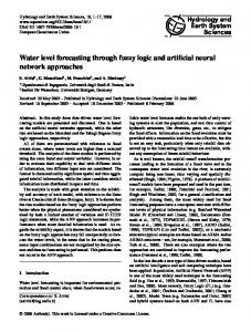
Figure 5. Trading performance of the different forecasting methodologies. Top: Excluding transactions costs. Bottom: Including transactions costs.
120
Operational Research. An International Journal / Vol.6, No.2 / May - August 2006
The profitability from trading based on the predictions of the global FNN model is depicted with the red line (Global FNN) in Fig. 5. As can be seen from Fig. 5, excluding transactions costs the FNN is capable of achieving a profit of 282.94 Euros over the 200 days of the test set, while including transactions costs reduces total profit to 109.57 Euros. Next, the results obtained by the k nearest neighbor regression method are presented. We experimented with all the integer values of k in the range [ 1,20]. The best performance was exhibited for k=5, and is illustrated with the black line (5 Nearest Neighbor) in Fig. 5. The 5 nearest neighbor method achieved a profit of 379.51 excluding transactions costs and 129.16 including transactions costs. Finally, the performance of the forecasting system based on the segmentation of the input using the UKW algorithm and utilizing an FNN to act as a local predictor for each cluster, is illustrated with the blue line (UKW FNN) in Fig. 5. This approach achieved the highest profit: in the absence of transactions costs, 472.16 Euros, and 235.54 including transactions costs.
3.3 Multiple Step Ahead Forecasting In [Pavlidis et al. (2005)b] we considered the problem of multiple-step-ahead forecasting. The time series considered was that of the Japanese Yen against the U.S. Dollar. The series consists of 1827 observations spanning a period of five years, from the 1st of January 1998 until the 1st of January of 2003. The series is freely available from the website www.oanda.com. The training set contained the first 1500 patterns, while the remaining patterns, covering approximately the final year of data, were assigned to the test set. The UKW algorithm was employed to compute the clusters present in the training set. Pattern n is of the form p , = [z ,..., z +d+h_1], n = 1,..., 1500, and h=2,5 represents the forecasting horizon. That is the values to be predicted [z +d,...,Zn+d+h_1] are components o f the pattern vectors employed by the UKW algorithm. The FNNs associated with each cluster were trained to minimize the mean squared error of onestep-ahead prediction. As an additional evaluation criterion, the performance of the FNNs on the task of two- and five-step-ahead prediction on the training set was monitored. Having trained all the FNNs for 100 epochs, their performance on the task of two- and five-step-ahead prediction was evaluated on the test set. For the clusters to which patterns from the test set were assigned, Tables 4 and 5 report the minimum (min), mean, and maximum (max) performance with respect to correct sign prediction. Also the standard deviation (st.dev), as well as, the performance of the FNN that managed the highest multiple-step-ahead sign prediction on the train set (best) are provided. The number of test patterns that were assigned to each cluster is indicated next to the cluster index. Due to space limitations, the results for one cluster containing four patterns from the test set are not reported in Table 4 for the two-stepahead problem, while for the five-step-ahead task the results for three clusters containing one, four and five patterns respectively are not reported in Table 5.
N. G. Pavlidis et al. / Financial Forecasting through Unsupervised Clustering and Neural Networks
121
Table 4. Resultsfor the problem of 2-step-aheadprediction Cluster 5:13 patterns
Cluster 9:60 patterns
min
mean
max
st.dev
best
AOBP
0.46
0.46
0.46
0
0.46
SCG
0.46
0.49
0.61
RProp
0.46
0.46
0.46
0 . 0 5 0.53 0
0.46
min
mean
max
st.dev
best
AOBP
0.51
0.57
0.61
0.03
0.6
SCG
0.46
0.5
0.58
0 . 0 3 0.58
RProp
0.43
0.47
0.48
0 . 0 1 0.48
Cluster 6:39 patterns
Cluster 10:23 patterns
min
mean
max
st.dev
best
min
mean
max
AOBP
0.46
0.56
0.61
0 . 0 5 0.46
AOBP 0.47
0.53
0.56
0 . 0 3 0.52
SCG
0.43
0.57
0.61
0 . 0 7 0.61
RProp
0.61
0.61
0.61
0
0.61
st.dev
best
SCG
0.47
0.54
0.56
0 . 0 3 0.56
RProp
0.52
0.54
0.6
0.03
Cluster 7:64 patterns
0.52
Cluster 11:25 patterns
min
mean
max
st.dev
best
AOBP
0.37
0.41
0.43
0.01
0.42
SCG
0.45
0.45
0.45
0
RProp
0.45
0.,45 0.45
0
min
mean
max
st.dev
best
AOBP
0.56
0.61
0.72
0.06
0.56
0.45
SCG
0.52
0.52
0.6
0.02
0.52
0.45
RProp
0.52
0.52
0.52
0
0.52
Cluster 8:42 patterns
Cluster 12:50 patterns
min
mean
max
st.dev
best
min
mean
max
st.dev
best
AOBP
0.38
0.46
0.5
0.04
0.38
AOBP 0.42
0.45
0.5
0.03
0.48
SCG
0.35
0.5
0.54
0.06
0.35
0.51
0.52
0.02
0.44
RProp
0.5
0.52
0.54
0 . 0 1 0.54
0.52
0.52
0
0.52
SCG
0.44
RProp 0 . 5 2
On the task o f two-step-ahead prediction (Table 4), no FNN was able to achieve a correct sign prediction exceeding 50% for the patterns that were classified to cluster 7. A similar behavior is observed for clusters 17, 18, 19, and 20 for t h e five-stepahead prediction task. On the other hand, the minimum correct sign prediction exceeds 50% for most training algorithms in clusters 10 and 11 o f Table 4 and clusters 14, 15, and 21 o f Table 5. It is important to note that the FNNs that achieved the best performance on the task o f two- and five-step-ahead prediction on the training set were rarely the ones that exhibited the highest performance on the test set.
122
Operational Research. An International Journal / Vol.6, No.2 / May - August 2006
Table 5. Resultsfor the problem of 5-step-ahead prediction V
Cluster 11:35 patterns
SCG p 0 . 4
0.46
0.46
0.41
0.46
/
min
mean
max
st.dev
best
AOBP
0.51
0.53
0.54
0.01
0.54
SCG
0.34
0.48
0.54
0.07
0.45
RProp
0.48
0.51
0.54
0.01
0.51
Cluster 12:17 patterns min
mean
max
st.dev
best
AOBP
0.35
0.42
0.52
0.07
0.52
SCG
0.17
0.27
0.35
0.05
0.29
RProp
0.17
0.33
0.52
0.13
0.52
Cluster 13:9 patterns min
mean max
st.dev
best
AOBP
0.22
0.24
0.33
0.04
0.22
SCG
0,22
0.23
0.33
0.03
0.22
RProp
0.22
0.26
0.33
0.05
0.33
Cluster 14:75 patterns min
mean
max
st.dev
best
0.54
0.56
0.57
0
0.56
0.49
0.55
0.58
0.02
0.49
R P r o p 0.54
0.56
0.58
0.01
0.57
AOBP SCG
I
Cluster 15:64 patterns min
mean max
st.dev
best
AOBP
0.59
0.6
0,6
0
0.59
SCG
0.57
0.6
0.6
0
0.6
RProp
0.56
0.6
0.62
0.01
0.59
Cluster 16:15 patterns
AOBP
RProP10.26
0.06
0.4
Cluster 17:16 patterns min
mean
max
st.dev
best
AOBP
0.25
0.25
0.25
0
0.25
SCG
0.18
0.4
0.5
0.12
0.18
RProp
0.18
0.35
0.5
0.11
0.18
Cluster 18:9 patterns min
mean max
st.dev
best
AOBP
0.33
0.33
0.33
0
0.33
SCG
0.11
0.13
0.33
0.07
0.11
RProp
0.11
0.18
0.33
0.07
0.11
Cluster 19:17 patterns min
mean max
st.dev
best
AOBP
0.35
0,39
0.41
0.02
0.41
SCG
0.17
0.23
0.29
0.02
0.23
RProp
0.23
0.32
0.41
0.04
0.41
Cluster 20:10 patterns min
mean max
st.dev
best
AOBP
0.2
0.26
0.3
0.05
0.2
SCG
0.2
0.24
0.4
0.06
0.3
RProp
0.2
0.26
0.3
0.05
0.3
Cluster 21:40 patterns min
mean max
st.dev
best
AOBP
0.55
0.55
0.55
0
0.55
min
mean
max
st,dev
best
SCG
0.55
0.58
0.6
0.01
0.55
0.46
0.46
0.46
0
0.46
RProp
0.57
0.6
0.62
0.0t
0.6
N. G. Pavlidis et al. / Financial Forecasting through Unsupervised Clustering and Neural Networks
123
Selecting among the trained FNNs for each cluster the one with the highest performance with respect to minimum, mean, maximum and highest multiple-stepprediction accuracy on the training set, respectively, we computed the mean forecasting performance achieved on the entire test set. These results are illustrated in Table 6 for the two- and five-step-ahead tasks. As expected the accuracy of the forecasts deteriorates as the forecasting horizon is expanded.
Table 6. Overall forecasting accuracy achieved by selecting the best performing FNN with respect to min, mean, max, and best, resj~ectively. min mean max best 2-step-ahead
0.51
0.53
0.575
0.55
5-step-ahead
0.48
0.51
0.56
0.51
Since the embedding dimension used to construct the input patterns for the FNNs acting as local predictors was five, to perform six-step-ahead prediction through the aforementioned approach, implies that all the elements of input vector are previous outputs of the model. In other words, the problem becomes one of iterated (closedloop) prediction. We have tested the performance of the system on this task, but the model fails to keep track of the evolution of the series. In effect beyond a certain number of iterated predictions the output of the model converges, to a constant value, implying that the system has been trapped in a fixed point. Enhancing the model so as to be able to overcome this limitation is a very interesting problem which we intend to address in future work.
4. Conclusions This paper presents a time series forecasting methodology which draws from the disciplines of chaotic time series analysis, clustering, and artificial neural networks. The methodology consists of four stages. Primarily the minimum dimension necessary for phase space reconstruction through time-delayed embedding is calculated using the method of false nearest neighbors. To identify neighborhoods in the state space, time delayed vectors are subjected to unsupervised clustering. Thus, the number of clusters present in a dataset is endogenously approximated. Subsequently, a different feedforward neural network is trained on each cluster to act as a local predictor for the corresponding subspace of the input space. The methodology is applied to generate one-step-ahead, as well as, multiple-step-ahead forecasts for different time series of daily spot foreign exchange rates of major currencies. The obtained experimental results are promising for the case of one-stepahead forecasting. A finding common to all the unsupervised clustering algorithms considered is the identification of regions characterized by substantially different predictability. This result highlights the importance of devising a scheme that will be capable of synthesizing the outcome of different algorithms to produce a satisfactory performance on a broader region of the input space.: Trading based on the signals
124
Operational Research. An International Journal / Vok4, No. 1 / January - April 2004
obtained through the proposed approach generates positive profit, despite the very simple nature of the trading rule applied and the inclusion of trading costs. As expected, multiple-step-ahead prediction is a considerably more difficult task. Indeed the mean performance of the methodology under examination marginally exceeds the benchmark of 50%. In future work the synthesis of the results of the different clustering algorithms to improve the forecasting performance in larger regions of the input space, will be considered. We also intend to address the issue of iterated prediction, by incorporating the test proposed by Diks et al. (1996) which provides a measure of the extent to which the developed prediction system accurately captures the attractor of the measured data [Bakker et al. (2000)]. We also intend to consider alternative neural network models like recurrent neural networks.
Acknowledgements The authors thank the European Social Fund (ESF), Operational Program for Educational and Vocational Training II (EPEAEK II) and particularly the Program PYTHAGORAS, for funding this work. This work was also supported in part by the "Karatheodoris" research grant awarded by the Research Committee of the University of Patras.
References Alevizos P., Boutsinas B., Tasoulis D.K., Vrahatis M.N. (2002). Improving the orthogonal range search k-windows clustering algorithm. Proceedings of the 14th IEEE International Conference on Tools with Artificial Intelligence, 239-245. Alevizos P.,Tasoulis D.K., Vrahatis M.N. (2004). Parallelizing the unsupervised kwindows clustering algorithm. Parallel Processing and Applied Mathematics (eds. R. Wyrzykowski, J. Dongarra, M. Paprzycki, and J. Wasniewski), SpringerVerlag, Lecture Notes in Computer Science vol. 3019, 225-232. Allen F., Karjalainen R. (1999). Using genetic algorithms to find technical trading rules. Journal of Financial Economics vol. 51,245-271. Bakker R., Schouten J.C., Giles C.L., Takens F., van den Bleek C.M. (2000). Learning of chaotic attractors by neural networks. Neural Computation vol. 12, 2355-2383. Bezdek J.C. (1981). Pattern recognition with fuzzy objective function algorithms, Kluwer Academic Publishers. Cao L. (2003). Support vector machines experts for time series forecasting. Neurocomputing vol. 51,321-329. Clerc M., Kennedy J. (2002). The particle swarm-explosion, stability, and convergence in a multidimensional complex space. IEEE Transactions on Evolutionary Computation vol. 6, 58-73. de Bodt E., Rynkiewicz J., and Cottrell M. (2001). Some known facts about financial data. Proceedings of European Symposium on Artificial Neural Networks (ESANN'2001), 223-236.
N. G. Pavlidis et al. / Financial Forecasting through Unsupervised Clustering and Neural Networks
125
Diks C., van Zwet W.R., Takens F., DeGoede J. (1996). Detecting differences between delay vector distributions. Physical Review E vol. 53, 2169--2176. Eberhart R.C., Simpson P., Dobbins R. (1996). Computational intelligence PC tools. Academic Press. Ester M., Kriegel H.P., Sander J., Xu X. (1996). A density-based algorithm for discovering clusters in large spatial databases with noise. Proceedings of the 2nd Int. Conf. on Knowledge Discovery and Data Mining, 226-231. Farmer J.D., Sidorowich J.J. (1987). Predicting chaotic time series. Physical Review Letters vol. 59, 845-848. Frankel J.A., Rose A.K. (1995). Empirical research on nominal exchange rates. Handbook of International Economics (eds. G. Grossman and K. Rogoff), Amsterdam, North-Holland, vol. 3, 1689-1729. Fraser A.M. (1989). Information and entropy in strange attractors. IEEE Transactions on Information Theory vol. 35,245-262. Fritzke B. (1995). A growing neural gas network learns topologies. Advances in Neural Information Processing Systems (eds. G. Tesauro, D.S. Touretzky, and T.K. Leen), MIT Press, Cambridge MA, 625-632. Giles L.C., Lawrence S., Tsoi A.H. (2001). Noisy time series prediction using a recurrent neural network and grammatical inference. Machine Learning vol. 44, 161-183. Hartigan J.A., Wong M.A. (1979). A k-means clustering algorithm. Applied Statistics vol. 28, 100-108. Hastie T., Tibshirani R., Friedman J. (2001). The elements of statistical learning. Springer-Verlag. Haykin S. (1999). Neural networks: A comprehensive foundation. New York: Macmillan College Publishing Company. Igel C., Husken M. (2000). Improving the Rprop learning algorithm. Proceedings of the Second International ICSC Symposium on Neural Computation (NC 2000) (H. Bothe and R. Rojas, eds.), ICSC Academic Press, 115-121. Kennel M.B., Brown R., Abarbanel H.D. (1992). Determining embedding dimension for phase--space reconstruction using a geometrical construction. Physical Review A vol. 45, 3403-3411. Keogh E, and Folias T. (2002). The UCR time series data mining archive. Kohonen T. (1997). Self-organized maps. Berlin: Springer. Magoulas G.D., Plagianakos V.P., Vrahatis M.N. (2001). Adaptive stepsize algorithms for on-line training of neural networks. Nonlinear Analysis: Theory Methods and Applications A vol. 47, 3425-3430. Meese R.A., Rogoff K. (1983). Empirical exchange rate models of the seventies: do they fit out-of-sample? Journal of International Economics vol. 14, 3-24. Meese R.A., Rogoff K. (1986). Was it real? the exchange rate-interest differential relation over the modem floating-rate period. The Journal of Finance vol. 43, 933948.
126
Operational Research. An international Journal / Vol.4, No. 1 / January - April 2004
Milidiu R.L., Machado R.J., Renteria R.-P. (1999). Time-series forecasting through wavelets transformation and a mixture of expert models. Neurocomputing vol. 28 145-156. Moller M. (1993). A scaled conjugate gradient algorithm for fast supervised learning. Neural Networks vol. 6, 525-533. Bank of International Settlements. (2001). Central bank survey of foreign exchange and derivative market activity in April 2001. Bank of International Settlements. Parsopoulos K.E., Vrahatis M.N. (2002). Recent approaches to global optimization problems through particle swarm optimization. Natural Computing vol. 12351306. Pavlidis N.G., Tasoulis D.K., Plagianakos V.P., Siriopoulos C., Vrahatis M.N. (2005). Computational intelligence methods for financial forecasting. Proceedings of the International Conference of Computational Methods in Sciences and Engineering (ICCMSE 2005) (ed. T.E. Simos), Lecture Series on Computer and Computational Sciences vol. 4, 1416-1419. Pavlidis N.G., Tasoulis D.K., Plagianakos V.P., Vrahatis M.N. (2005). Time series forecasting methodology for multiple-step-ahead prediction. Proceedings of IASTED International Conference on Computational Intelligence (CI2005), 456461. Pavlidis N.G., Tasoulis D.K., Plagianakos V.P., Vrahatis M.N. Computational intelligence methods for financial time series modeling. International Journal of Bifurcation and Chaos (in press). Pinkus A. (1999). Approximation theory of the MLP model in neural networks. Acta Numerica, 143-195. Plagianakos V.P., Magoulas G.D., Vrahatis M.N. (2000). Global learning rate adaptation in on--line neural network training. Proceedings of the Second International ICSC Symposium on Neural Computation (NC 2000). Plagianakos V.P., Vrahatis M.N. (2002). Parallel evolutionary training algorithms for "hardware-friendly" neural networks. Natural Computing vol. 1,307-322. Principe J.C., Wang L., Motter M.A. (1998). Local dynamic modeling with selforganizing maps and applications to nonlinear system identification and control. Proceedings of the IEEE vol. 86, 2240-2258. Refenes A.N., Holt W.T. (2004). Forecasting volatility with neural regression: A contribution to model adequacy. IEEE Transactions on Neural Networks vol. 12, 850-864. Riedmiller M., Braun H. (1993). A direct adaptive method for faster backpropagation learning: The Rprop algorithm. Proceedings of the IEEE International Conference on Neural Networks, San Francisco, CA, 586-591. Sandberg I.W., Xu L. (1997). Uniform approximation and gamma networks. Neural Networks vol. 10, 781-784. Sandberg I.W., Xu L. (1997). Uniform approximation of multidimensional myopic maps. IEEE Transactions on Circuits and Systems I: Fundamental Theory and Applications vol. 44, 477-485.
N. G. Pavlidis et al. / Financial Forecasting through Unsupervised Clustering and Neural Networks
127
Sander J., Ester M., Kriegel H.-P., Xu X. (1998). Density-based clustering in spatial databases: The algorithm gdbscan and its applications. Data Mining and Knowledge Discovery vol. 2, 169-194. Sfetsos A, Siriopoulos C. (2004). Time series forecasting with a hybrid clustering scheme and pattern recognition. IEEE Transactions on Systems, Man, and Cybernetics Part A: Systems and Humans vol. 34, 399-405. Storn R., Price K. (1997). Differential evolution - a simple and efficient adaptive scheme for global optimization over continuous spaces. Journal of Global Optimization vol. 11,341-359. Sutton R.S., Whitehead S.D. (1993). Online learning with random representations. Proceedings of the Tenth International Conference on Machine Learning, Morgan Kaufmann, 314-321. Takens F. (1981). Detecting strange attractors in turbulence. Dynamical Systems and Turbulence (eds. D.A. Rand and L.S. Young ), Lecture Notes in Mathematics, vol. 898, Springer, 366-381. Tasoulis D.K., Vrahatis M.N. (2004). Unsupervised distributed clustering. IASTED International Conference on Parallel and Distributed Computing and Networks, 347-351. Tasoulis D.K., Vrahatis M.N. (2005). Unsupervised clustering on dynamic databases. Pattern Recognition Letters vol. 26, 2116-2127. Vrahatis M.N., Boutsinas B., Alevizos P., Pavlides G. (2002). The new k-windows algorithm for improving the k-means clustering algorithm. Journal of Complexity vol. 18, 375-391. Walczak S., (2001). An empirical analysis of data requirements for financial forecasting with neural networks. Journal of Management Information Systems vol. 17, 203-222. Weigend A.S., Mangeas M., Srivastava A.N. (1995). Nonlinear gated experts for time series: Discovering regimes and avoiding overfitting. International Journal of Neural Systems vol. 6, 373-399. White H. (1990). Connectionist nonparametric regression: Multilayer feedforward networks can learn arbitrary mappings. Neural Networks vol. 3,535-549. Wilson D.R., Martinez T.R. (1997). Improved heterogeneous distance functions. Journal of Artificial Intelligence Research vol. 6, 1-34. Yao J., Tan C.L. (2000). A case study on using neural networks to perform technical forecasting of forex. Neurocomputing vol. 34, 79-98.