Finding a Maximum Independent Set in a Sparse Random Graph pc0

Finding a Maximum Independent Set in a Sparse Random Graph Uriel Feige

∗

Eran Ofek

†

December 23, 2007

Abstract We consider the problem of finding a maximum independent set in a random graph. The random graph G, which contains n vertices, is modelled as follows. Every edge is included independently with probability nd , where d is some sufficiently large constant. Thereafter, for some constant α, a subset I of αn vertices is chosen at random, and all edges within this subset are removed. In this model, the planted independent set I is a good approximation for the maximum independent set Imax , but both I \ Imax and Imax \ I are likely to be nonempty. We present a polynomial time algorithms that with high probability (over the random choice of random graph G, and without p c being given the planted independent set I) 0 finds the maximum independent set in G when α ≥ , where c0 is some sufficiently large constant d independent of d.

1

Introduction

Let G = (V, E) be a graph. An independent set I is a subset of vertices which contains no edges. The problem of finding a maximum size independent set in a graph is a fundamental problem in Computer Science and it was among the first problems shown to be NP-hard [18]. Moreover, Hastad shows [15] that for any ² > 0 there is no n1−² approximation algorithm for the maximum independent set problem unless NP=ZPP. The best approximation ratio currently known for maximum independent set [7] is O(n(log log n)2 /(log n)3 ). In light of the above mentioned negative results, we may try to design a heuristic that performs well on typical instances. Karp [17] proposed trying to find a maximum independent set in a random graph. However, even this problem appears to be beyond the capabilities of current algorithms. For example, let Gn,1/2 denote the random graph on n vertices obtained by choosing randomly and independently each possible edge with probability 1/2. The size of the maximum independent set in a random Gn,1/2 graph is almost surely 2(1 + o(1)) log2 n. A simple greedy algorithm almost surely finds an independent set of size log2 n [14]. However, there is no known polynomial time algorithm that almost surely finds an independent set of size (1 + ²) log2 n (for any ² > 0). To further simplify the problem, Jerrum [16] and Kucera [19] proposed a planted model Gn,1/2,k in which a random graph Gn,1/2 is chosen and then a clique of size k is randomly placed in the graph. (A clique in a graph G is an independent set in the edge complement of G, and hence all algorithmic results that apply to one of the problems apply to the other.) Alon, Krivelevich and Sudakov √ [2] gave an algorithm based on spectral techniques that almost surely finds the planted clique for k = Ω( n). More generally, one may extend the range of parameters of the above model by planting an independent set in Gn,p , where p need not be equal to 1/2, and may also depend on n. The Gn,p,α model is as follows: n vertices are partitioned at random into two sets of vertices, I of size αn and C of size (1 − α)n. No edges are placed within the set I, thus making it an independent set. Every other possible edge (with at least one endpoint not in I) is added independently at random with probability p. The goal of the algorithm, given the input G (but without being given the partition into I and C) is to find a maximum independent set. Intuitively, as α becomes ∗ Department of Computer Science and Applied Mathematics, the Weizmann Institute, Rehovot 76100, Israel. [email protected] † Schema, Herzlia 46905, Israel. [email protected]

1

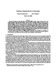
smaller the size of the planted independent is closer to the probable size of the maximum independent set in Gn,p and the problem becomes harder. We consider values of p as small as d/n where d is a large enough constant. A difficulty that arises in this sparse regime (i.e. when d is constant) is that the planted independent set I is not likely to be a maximum independent set. Moreover, with high probability I is not contained in a maximum independent set of G. For example, there are expected to be e−d n vertices in C of degree one. It is very likely that two (or more) such vertices v, w ∈ C will have the same neighbor, and that it will be some vertex u ∈ I. This implies that every maximum independent set will contain v, w and not u, and thus I contains vertices that are not contained in the maximum independent set.

C

I

w v

u

Figure 1: The vertex u ∈ I is not contained in any maximum independent set because no other edges touch v, w. A similar argument shows that there are expected to be e−Ω(d) n isolated edges. This implies that there will be an exponential number of maximum independent sets.

1.1

Our result

Our main result is summarized in the following theorem. Theorem 1.1. There is a polynomial time algorithm that almost surely finds the maximum independent set p of a graph G selected at random from the distribution Gn, d ,α , when d > d0 and α ≥ c0 /d (d0 , c0 are some n universal constants). The parameter d can also be an increasing function of n. The bulk of the paper is devoted to proving the above theorem. To simplify the presentation of the proof it will be convenient to assume upper bounds on d and on α, namely d < n1/40 and α < 1/3. These upper bounds do not limit the generality of our results, because when d or α exceed these uppers bounds the proof becomes simpler (see later discussions in the paper).

1.2

Related work

√ For p = 1/2, α = Ω(1/ n), Alon, Krivelevich and Sudakov [2] gave an efficient spectral algorithm which almost surely finds the planted independent set. For the above mentioned parameters the planted independent set is likely to be the unique maximum independent set. A few papers deal with semi-random models which extend the planted model by enabling a mixture of random and adversarial decisions. Feige and Kilian [8] considered the following model: a random Gn,p,α graph is chosen, then an adversary may add arbitrarily many edges between I and C, and make arbitrary changes (adding or removing edges) inside C. For any constant α > 0 they give a heuristic that almost surely outputs a list of independent sets containing the planted independent set, whenever p > (1 + ²) ln n/αn (for any ² > 0). The planted independent set may not be the only independent set of size αn since the adversary has full control over the edges inside C. Possibly, this makes the task of finding the planted independent set 2

harder. In [9] Feige and Krauthgamer considered a less adversarial semi-random model in which an adversary is allowed to add edges to a random Gn, 12 , √1 graph. Their algorithm almost surely extracts the planted n

independent set and certifies its optimality. Coja-Oghlan [5] considered similar semi-random variants of random Gn,p,√c/pn graphs, with ln(n)2 /n < p < 0.99 (and c a sufficiently large constant). He shows among other things that in most such graphs a maximum independent set can be found in polynomial time. Extracting from the above discussion the known previous results on planted independent set models (and ignoring issues such as handling semirandom p instances), we see that the same tradeoff between d and α as claimed in the current paper (namely, α ≥ c0 /d) was previously established for the case d = n/2 (first p in [2], 2 and then again in [9]), and then extended all the way down to d = ln n in [5]. The condition α ≥ c0 /d is needed mainly to ensure that the effect of planting the independent set I shows up in the spectrum of the adjacency matrix of the graph. For the previous range of parameters, the planted independent set is likely to be the maximum independent set in the graph. In this paper we address the case that d is a (sufficiently large) constant, which introduces difficulties not present in earlier work, mainly due to the fact that the planted independent set is likely not to be the maximum independent set. Heuristics for optimization problems different than max independent set will be discussed in the following section. 1.2.1

Technique and outline of the algorithm

Our algorithm builds on ideas from the algorithm of Alon and Kahale [1], which was used for recovering a planted 3-coloring in a random graph. The algorithm that we propose has four phases, and is sketched below. This overall structure is similar to the structure of the algorithm of [1], but phases 3 and 4 include ingredients that are different than those of [1]. These differences are discussed towards the end of this section. 1. Get a coarse approximation I 0 , C 0 of I, C with |C M C 0 | + |I M I 0 | < spectral techniques.

1 60 |I|.

This phase is based on

2. Reduce the error in the approximation by using an iterative procedure based on the number of neighbors that each vertex has in I 0 . The error term |C M C 0 | + |I M I 0 | is reduced to at most n/d18 . 3. Commit to placing certain vertices of I 0 in the final independent set. This is done by moving vertices from I 0 and C 0 to OU T (a new set), and committing to placing the remaining part of I 0 in the final independent set. The choice of vertices to move to OU T depends on their degree into I 0 . When this process ends, I 0 is an independent set, every vertex of C 0 has at least 4 edges to I 0 and no vertex of I 0 has edges to OU T . Using the fact that sparse random graphs (almost surely) have no small dense sets, it will be shown that I 0 ⊆ Imax and also that OU T is rather small. 4. Extend the independent set I 0 optimally using the vertices of OU T . This is done by finding a maximum independent set among the vertices of OU T and adding it to I 0 . The structure of OU T will be simple enough so that a maximum independent set can be efficiently found. The proof is based to a large extent on the fact that OU T is small. If vertices of OU T were chosen independently at random from the input graph G, then it would have been easy to show that all connected components in OU T are very small (say, of size O(log n)), and then a maximum independent set in OU T can be found in time polynomial in n (even by exhaustive search). However, OU T is a result of a deterministic process applied to G, which makes the analysis of its structure considerably more difficult. The technique of [1] was implemented successfully on various problems in the planted model: planted hypergraph coloring, planted 3-SAT, planted 4-NAE, min-bisection (by Chen and Frieze [4], Flaxman [12], Goerdt and Lanka [13], Coja-Oghlan [6] respectively). Perhaps the work closest in nature to the work in the current paper is that of Amin Coja-Oghlan [6] on finding a bisection in a sparse random graph. Both in our work and in that of [6], one is dealing with an optimization problem, and the density of the input graph is such that the planted solution is not an optimal solution. The algorithm for bisection in [6] is based on spectral techniques, and has the advantage that it 3

provides a certificate showing that the solution that it finds is indeed optimal. We do not address the issue of certification in this paper. In [6] the random instance is generated as follows. The vertices of the graph are partitioned into two classes of equal size randomly. Then the edges are inserted: edges inside the two classes with probability p0 and edges crossing the partition with probability p independently. Intuitively, as p0 − p becomes smaller, the problem becomes harder. Denote by d1 = np0 /2, d2 = np/2 the expected degree of a vertex into its own class and into √ the other class respectively. The algorithm in [6] is proven to succeed (almost surely) whenever d1 − d2 ≥ c0 d1 log d1 . In our independent set model the problem becomes harder as αd becomes smaller. If we denote by d˜1 = d, d˜2 = (1 − α)d the expected degrees ofpa vertex in C and I respectively, then our algorithm (almost surely) succeeds whenever d˜1 − d˜2 = αd˜1 ≥ c0 d˜1 . We remark that a significant source q for complications in our algorithm and its analysis comes from a tightening of the parameters, saving a log d˜ factor in the size of α. A preliminary version of this work (see [11]) presents a q simpler algorithm but requires αd˜1 ≥ c0 d˜1 log d˜1 An important difference between planted models for independent set and those for other problems such as 3-coloring and min-bisection is that in our case the planted classes I, C are not symmetric. The lack of symmetry between I and C makes some of the ideas used for the more symmetric problems insufficient. In the approach of [1], a vertex is removed from its current color class and placed in OU T if its degree into some other current color class is very different than what one would typically expect to see between the two color classes. This procedure is shown to ”clean” every color class C from all vertices that should have been from a different color class, but were wrongly assigned to class C in phase 2 of the algorithm. (The argument proving this goes as follows. Every vertex remaining in the wrong color class by the end of phase 3 must have many neighbors that are wrongly assigned themselves. Thus the set of wrongly assigned vertices induces a small subgraph with large edge density. But G itself does not have any such subgraphs, and hence by the end of phase 3 it must be the case that all wrongly assigned vertices were moved into OU T .) It turns out that this approach works well when classes are of similar nature (such as color classes, or two sides of a bisection), but does not seem to suffice in our case where I 0 is supposed to be an independent set whereas C 0 is not. Specifically, the set I 0 might still contain wrongly assigned vertices, and might not be a subset of a maximum independent set in the graph. Under these circumstances, phase 4 will not result in a maximum independent set. Our solution to this problem involves the following aspects, not present in previous work. In phase 3 we remove from I 0 every vertex that has even one edge connecting it to OU T . This adds more vertices to OU T , and makes the connected components in OU T larger. We do not attempt to analyze the maximum size of connected components in OU T , which is a key ingredient in previous approaches. Instead, we analyze the 2-core of OU T and show that the 2-core has no large components. Then, in phase 4, we use dynamic programming to find a maximum independent set in OU T , and use the special structure of OU T to show that the algorithm runs in polynomial time.

1.3

Notation

Let G = (V, E) and let U ⊂ V . The subgraph of G induced by the vertices of U is denoted by G[U ]. When the set of edges used is clear from the context, we will use deg(v)U to denote the degree of a vertex v into a set U ⊂ V . To specify exactly the set of edges used, we use degE (v)U which is the degree of a vertex v into a set U induced by the set of edges E. We use Γ(U ) to denote the vertex neighborhood of U ⊂ V (excluding U ). The parameter d (specifying the expected degree in the random graph G) is assumed to be sufficiently large, and some of the inequalities that we shall derive implicitly use this assumption, without stating it explicitly. The term with high probability (w.h.p.) is used to denote a sequence of probabilities that tends to 1 as n tends to infinity.

2

The Algorithm

The p first step of the algorithm is tailored to deal with the case that α is small. When α is large (in fact, α > 100 log d/d suffices), the combination of step 1 and step 2 can be replaced by a simpler step based on 4

partitioning the vertices according to their degrees (see Section 3.2 for details). Hence we shall assume here that α ≤ 1/3, and this will somewhat simplify the presentation of the algorithm and its analysis. Furthermore, we assume for simplicity that the values of the parameters α, d are given as input to the algorithm. This assumption can be avoided by enumerating all possible values of α, d (actually we need only a good approximations of α, d). Algorithm F indIS(V, E) 1. Let A0 be the adjacency matrix of the graph induced by removing from G all vertices of degree > 5d. Compute the eigenvector of the most negative eigenvalue of A0 , denoted by vn0 . Sort the vertices of V 0 in order of the value of the corresponding entry in vn0 , breaking ties arbitrarily. Let I1 be either the first αn vertices in this sorted order or the last αn vertices. (To choose among the above two options, find a maximal matching in each of the two possible induced graphs G(I1 ), and pick the option for which the maximal matching found is smaller.) Set C1 = V \ I1 . 2. Set C20 = C1 , I20 = I1 . Iterate j = 1, 2, .., log n: for every vertex v: if deg(v)I j−1 < αd/2 then v ∈ I2j , otherwise v ∈ C2j . 2

3. (a) Set I3 =

I2log n ,

C3 =

C2log n ,

OU T3 = ∅.

(b) For every edge (u, v) such that both u, v are in I3 , move u, v to OU T3 . (c) A vertex v ∈ C3 is removable if deg(v)I3 < 4. Iteratively: find a removable vertex v and move it from C3 to OU T3 . If v has neighbors in I3 , move these neighbors from I3 to OU T3 . 4. Find a maximum independent set in G[OU T3 ] (this will be shown to be doable in polynomial time, see Corollary 3.4). Output the union of this independent set and I3 . Figure 2 depicts the situation after step 3 of the algorithm is done. At that point, I3 is an independent set, there are no edges between I3 and OU T3 , and every vertex v ∈ C3 has at least four neighbors in I3 .

C3

I3

3
1 − o(n− d )). 3. There is no C 0 ⊆ C such that n/2d5 ≤ |C 0 | ≤

2n log d d

and |Γ(C 0 ) ∩ I| ≤ |C 0 |.

Corollary 3.6. Let G be a graph which has the property from Lemma 3.5 part 1. Let A, B be any two disjoint sets of vertices each of size smaller than n/d5 . If every vertex of B has at least 2 edges going into A, then |A| ≥ |B|/2. Proof. Assume for the sake of contradiction that |A| = δ|B| for some 0 < δ < 1/2. The number of internal edges of A ∪ B is at least 2|B| > 34 (1 + δ)|B| = 43 |A ∪ B|. The last inequality contradicts part 1 of Lemma 3.5. The following lemma bounds the number of vertices whose degree largely deviates from its expectation. Lemma 3.7. Let d < n1/40 . With probability > 1 − e−n

0.1

:

1. There are at most n/d21 vertices in C whose degree into I is < 0.9αd.

6

2. There are at most 3e−d dn edges that contain a vertex with degree at least 3d. Lemma 3.8. W.h.p. the size of a maximum independent set in G[C] is
n1/40 , the planted independent set is almost surely the unique maximum independent set, and can be found using algorithms described in earlier work [2, 5]. When α ≥ 1/3 step 1 of the algorithm can be replaced by the following simpler step: put in I1 all the vertices of degrees < (1 − α/2)d and the rest of the vertices in C1 . A simple argument (similar to the proof of Lemma 3.7) shows that in this case w.h.p. |I M I1 | < |I|/60 (see [11] for more details). Hence when analyzing step 1 of the algorithm (proving that w.h.p. |I M I1 | < |I|/60), we will without loss of generality limit the range of α to α < 1/3. We will show that if G is good then steps 1, 2, 3 of the algorithm give a very good approximation of I, C. 3.2.1

An aid in the analysis

For the sake of the analysis, we introduce Definition 3.11. This definition identifies certain key sets of vertices in the graph (V2 and V3 ). Definition 3.11 involves an algorithm that has complete knowledge of the planted independent set I. To avoid the possibility of confusion, let us stress here that this algorithm is not part of the algorithm F indIS, and moreover, the sets V2 and V3 are neither given to nor computed by algorithm F indIS. Definition 3.11. Given a graph G = (V, E) with an independent set I (and a corresponding vertex cover C = V \ I) the P-core of G is a subset of V which is extracted using the following steps. CR0:

Initialization: Iteratively:

CR1:

Initialization: Iteratively:

V2 = I ∪ {v ∈ C | deg(v)I ≥ 0.9αd}. (i) if there is v ∈ I ∩ V2 with deg(v)V \V2 > αd/4 remove v from V2 . (ii) if there is v ∈ C ∩ V2 with deg(v)I∩V2 < 0.8αd, remove v from V2 . V3 = V2 , remove from V3 all the vertices of V3 ∩ I that have edges to V \ V3 . find a vertex v ∈ V3 ∩ C with deg(v)V3 ∩I < 4, remove v and its neighbors in I from V3 . 7

The P-core of G is defined to be V3 . We use P-core to denote V \ P-core. The sets V2 and V3 have certain structural properties, as defined in Definition 3.11. We shall also need the fact that if G is a good graph (in the sense of Definition 3.10) then almost all vertices of G are in V2 and in V3 . Lemma 3.12. For a good graph G, the following hold: 1. |V \ V2 | < n/d20 (where V2 = CR0(G)). 2. |P-core| < n/d18 . Proof. Since G is good, after setting V2 = I ∪ {v ∈ C | deg(v)I ≥ 0.9αd} (and before the iterations of CR0) it holds that |V \ V2 | < n/d21 (see Lemma 3.7 part 1). In the iteration process, every vertex that we remove from V2 contributes at least 0.1αd edges to V \ V2 . If the iteration steps are repeated too many times, V \ V2 will become dense. Assume by contradiction that at some point the set V \ V2 doubled its size (when we compare it to the size before the first iteration). At this point it contains at least 12 |V \ V2 |0.1αd edges and its size is at most 2n/d21 , which contradicts the definition of good G (see Lemma 3.5 part 2). This proves item 1 of the lemma. We now prove item 2 of the lemma. Initially V3 = V2 , at this point |V \ V3 | ≤ n/d20 (using part 1 of this Lemma). We then remove from V3 all the vertices of I that have edges to V \ V3 . Doing so, we loose at most 3dn/d20 + 3de−d n vertices (see the definition of good G in Lemma 3.7 part 2; for a random G this 0.1 happens with probability > 1 − e−n ). At this point (just before the iteration steps) |V \ V3 | ≤ 4n/d19 . We now begin the iteration process. In every iteration we remove a vertex u of V3 ∩ C whose degree into V3 ∩ I became < 4 (we also remove its neighbors from V3 ∩ I). Note that after the initialization of CR1 the degree of u into V3 ∩ I was ≥ 0.8αd. It follows that after removing u and its neighbors from V3 ∩ I there are at least 0.8αd additional edges in V \ V3 . If the iteration step is repeated too many times the set V \ V3 will become too dense. Assume by contradiction that at some point (for the first time during the iterations) |V \ V3 | doubled its size when compared to the size of V3 \ V before the first iteration. At this point the number of edges inside V \ V3 is at least 21 |V \ V3 | · 14 · 0.8αd. Moreover, the size of V \ V3 at this point is ≤ 8n/d19 + 3 < n/d5 . √This can not happen in a good G (see Lemma 3.5 part 2; for a random G this happens with probability o(n− d )). We conclude that |V \ V3 | < n/d18 . Remark: The reader can verify by inspection that those√properties of good graphs that are used in the proof of Lemma 3.12 hold with probability at least 1 − o(n− d ) (for a random graph taken from Gn,d/n,α ). √ Hence Pr[P-core < n/d18 ] > 1 − o(n− d ). 3.2.2

Analysis of Step 1.

Lemma 3.9 states that the spectral phase of the algorithm (step 1) is likely to give a good approximation of the planted independent set. The proof of Lemma 3.9 follows from known principles, but it is rather involved. It is given in Section 4.2. 3.2.3

Analysis of Step 2.

In this section, we assume that G is good (as in Definition 3.10). The approximation I1 , C1 serves as a bootstrap for the “error reduction” done at step 2. In Lemma 3.13 we show that step 2 significantly reduces the error term i.e. |I2 M I| < n/d20 < |I|/d19 . The idea of the proof is as follows. Recall that in Lemma 3.12 we showed that the set V2 = CR0(G) from Definition 3.11 is of size > (1 − 1/d20 )n. Here we will use the assumption that G is good to show that every iteration of step 2 of F indIS reduces the number of errors (with respect to I, C) in V2 by a factor of 2. It then follows that after step 2 is done, all the vertices of V2 are assigned correctly. Lemma 3.13 (Error reduction). Let G be a good graph, V2 = CR0(G) and I2 = I2log n from step 2 of F indIS(G). Then V2 ∩ (I M I2 ) = ∅ and |I2 M I| ≤ n/d20 . 8

Proof. When step CR0 ends, every vertex of C ∩ V2 has at least 0.8αd edges to I ∩ V2 and every vertex of I ∩ V2 has at most αd/4 edges to V \ V2 . For each iteration i of step 2 of F indIS(G), define the respective “error” Ei to be the set of those vertices of V2 that are assigned incorrectly, namely, Ei = V2 ∩ (I2i M I). We will show that each iteration of step 2 of F indIS(G) reduces the error by a factor of at least 2. This is based on the fact (to be shown shortly) that every vertex of Ei has at least αd/4 edges to Ei−1 . Based on this fact we show that an event |Ei | ≥ |Ei−1 |/2 would lead to a contradiction. Fix Ei0 to be any subset of Ei whose size is |Ei−1 |/2 (if |Ei−1 | is odd we take a subset of size d|Ei−1 |/2e and essentially the same argument goes through). The set Ei0 ∪ Ei−1 is of cardinality ≤ 23 |Ei−1 | and it contains at least αd 4 |Ei−1 |/2 edges. This contradicts the definition of good G as |Ei−1 | ≤ |E0 | ≤ αn/60 (see Lemma 3.5 part 2, note that |Ei0 ∪ Ei−1 | ≤ 23 |Ei−1 | ≤ αn/40). We now show that each vertex of Ei has at least αd/4 edges to Ei−1 . case 1: v ∈ Ei−1 ∩ Ei (either v ∈ I ∩ C2i−1 or v ∈ C ∩ I2i−1 ): If v ∈ I ∩ C2i−1 (and v ∈ Ei ) then in round i − 1 it has at least αd/2 neighbors in I2i−1 , these neighbors are in C ∩ I2i−1 since v ∈ I. At least αd/4 of these neighbors are in V2 since v has at most αd/4 edges to V \ V2 (because v ∈ I ∩ V2 ). Thus v has > αd/4 neighbors in Ei−1 . If v ∈ C ∩ I2i−1 (and v ∈ Ei ) then in round i − 1 it has at most αd/2 neighbors in I2i−1 . Since v ∈ V2 ∩ C it has 0.8αd neighbors in I ∩ V2 , thus at least 0.3αd of them are in I ∩ C2i−1 ⊆ Ei−1 . case 2: v ∈ Ei \ Ei−1 : If v ∈ Ei \ Ei−1 ∩ I then v was moved from I2i−1 to C2i , therefore it has at least αd/2 neighbors in I2i−1 ∩ C. Among them at least αd/4 belong to V2 because v has at most αd/4 edges to V \ V2 . If v ∈ Ei \ Ei−1 ∩ C then v was moved from C2i−1 to I2i , therefore it has at most αd/2 neighbors in I2i−1 . Since v ∈ V2 ∩ C it has at least 0.8αd neighbors in I ∩ V2 , among which at least 0.3αd are in I ∩ C2i−1 ⊆ Ei−1 . It follows that when step 2 is done all the vertices of V2 are correctly assigned by the algorithm. It then follows that |I2 M I| ≤ |V \ V2 | ≤ n/d20 , where the last inequality follows from Lemma 3.12 part 1. 3.2.4

Analysis of Step 3.

So far we have shown that at most n/d20 vertices of I2 , C2 are wrongly assigned (with respect to I, C). The goal of step 3 is to “clean” I2 , C2 yielding I3 , C3 that can be extended into an optimal solution. Before showing that I3 ⊆ Imax (for some maximum independent set Imax ) we show that the process of “cleaning” in step 3 does not move too many vertices to OU T3 . This will be used later for proving that I3 ⊆ Imax . For the following lemma, recall the notion of P-core from Definition 3.11. Lemma 3.14. Let G be a good graph and let OU T3 be the outcome of step 3 of F indIS(G). Then OU T3 ⊆ P-core, and OU T3 < n/d18 . Proof. As OU T3 = I3 ∪C3 (where I3 , C3 are from step 3 of F indIS(G)) it is enough to show that V3 ⊆ I3 ∪C3 . Immediately after step 3a it holds that I3 ∪ C3 = V and thus V3 ⊆ I3 ∪ C3 . We will show that this is kept during steps 3b, 3c. Initially (at CR1) V3 = V2 . Removing from V3 all the vertices of V3 ∩ I that have edges to V \ V3 ensures that there are no edges between vertices of V3 ∩ I and vertices which were assigned incorrectly (all the vertices of V3 ⊆ V2 are correctly assigned after step 2 of the algorithm, see Lemma 3.13 part 2). Thus, step 3b of the algorithm does not touch any vertex of V3 because it removes only edges that contain at least one wrongly assigned endpoint. Finally, the iteration process of CR1 ensures that every vertex of V3 ∩ C has at least 4 edges to vertices in V3 ∩ I. Since V3 is a subset of I3 ∪ C3 at the beginning of step 3c and there are no wrongly assigned vertices in V3 , during step 3c there will never be a vertex of V3 ∩ C that has fewer than 4 edges to vertices of V3 ∩ I. We conclude that V3 ⊆ I3 ∪ C3 at the end of step 3. Combining with Lemma 3.12 part 2, we deduce that with high probability OU T3 < n/d18 . As |I3 M I| < |I2 M I| + |OU T3 |, using Lemmas 3.13, 3.14 we deduce: Corollary 3.15. For a good G, it holds that |I3 M I| < 2n/d18 . It turns out that I3 , C3 is also a good approximation of Imax , Cmax (Imax is any maximum independent set, Cmax = V \ Imax ). 9

Lemma 3.16. For a good G it holds |I3 M Imax | < n/d5 . Proof. |Imax M I3 | ≤ |Imax M I| + |I M I3 | 18

By Corollary 3.15 |I3 M I| < n/d . It remains to bound |Imax M I|: |Imax M I| = |Imax \ I| + |I \ Imax | ≤ 2|Imax \ I| = 2|Imax ∩ C| Imax = (Imax ∩ I) ∪ (Imax ∩ C). One can always replace Imax ∩ C with Γ(Imax ∩ C) ∩ I to get an independent d set (Imax ∩ I) ] (Γ(Imax ∩ C) ∩ I). The size of a maximum independent set of C is < 2n log (as G is good, d see Lemma 3.8). This upper bounds |Imax ∩ C|. From Lemma 3.5 part 3 if |Imax ∩ C| > n/(2d5 ) then |Γ(Imax ∩ C) ∩ I| > |Imax ∩ C| which contradicts the maximality of Imax . At this point (for a good G) we know that I3 , C3 have the following two properties: (i) the error term |(I3 ∩ Cmax ) ∪ (Imax ∩ C3 )| ≤ |Imax M I3 | < n/d5 . (ii) I3 is an independent set and every vertex of C3 has at least 4 neighbors in I3 . The above two properties and the fact that G is good imply that I3 ⊆ Imax . This is proven in the following Lemma. Lemma 3.17 (Extension Lemma). Let Im be any independent set of G (the reader may think of Im as Imax ) M and let Cm = V \ Im . Let I 0 , C 0 , OU T 0 be an arbitrary partition of V for which I 0 is an independent set. If the following hold: 1. |(I 0 ∩ Cm ) ∪ (Im ∩ C 0 )| < n/d5 . 2. Every vertex of C 0 has at least 4 neighbors in I 0 . None of the vertices of I 0 have edges to OU T 0 . 3. The graph G has no small dense subsets as described in Lemma 3.5 part 1. M

then there exists an independent set Inew (and Cnew = V \ Inew ) such that I 0 ⊆ Inew , C 0 ⊆ Cnew and |Inew | ≥ |Im |. Proof. If we could show that on average a vertex of U = (I 0 ∩ Cm ) ∪ (Im ∩ C 0 ) contributes at least 4/3 internal edges to U , then U would form a small dense set that contradicts Lemma 3.5. This would imply that U = (I 0 ∩ Cm ) ∪ (Im ∩ C 0 ) is the empty set, and we could take Inew = Im in the proof of Lemma 3.17. The proof below extends this approach to cases where we cannot take Inew = Im . Every vertex v ∈ C 0 has at least 4 edges into vertices of I 0 . Since Im is an independent set it follows that every vertex of Im ∩ C 0 has at least 4 edges into I 0 ∩ Cm . To complete the argument we would like to show that every vertex of I 0 ∩ Cm has at least 2 edges into Im ∩ C 0 . However, some vertices v ∈ I 0 ∩ Cm might have less than two neighbors in Im ∩ C 0 . In this case, we will modify Im to get an independent set Inew (and M Cnew = V \ Inew ) at least as large as Im , for which every vertex of I 0 ∩ Cnew has 2 neighbors in Inew ∩ C 0 . This is done iteratively; after each iteration we set Im = Inew , Cm = Cnew . Consider a vertex v ∈ (I 0 ∩ Cm ) with deg(v)Im ∩C 0 < 2: • If v has no neighbors in Im ∩ C 0 , then define Inew = Im ∪ {v}. Inew is an independent set because v (being in I 0 ) has no neighbors in I 0 nor in OU T 0 . • If v has only one edge into w ∈ (Im ∩ C 0 ) then define Inew = (Im \ {w}) ∪ {v}. Inew is an independent set because v (being in I 0 ) has no neighbors in I 0 nor in OU T 0 . The only neighbor of v in Im ∩ C 0 is w. The three properties are maintained also with respect to Inew , Cnew (replacing Im , Cm ): properties 2, 3 are independent of the sets Im , Cm and property 1 is maintained since after each iteration it holds that |(I 0 ∩ Cnew ) ∪ (Inew ∩ C 0 )| < |(I 0 ∩ Cm ) ∪ (Im ∩ C 0 )|. When the process ends, let U denote (I 0 ∩ Cm ) ∪ (Im ∩ C 0 ). Each vertex of I 0 ∩ Cm has at least 2 edges into Im ∩ C 0 , thus |Im ∩ C 0 | ≥ 12 |I 0 ∩ Cm | (see Corollary 3.6). Each vertex of Im ∩ C 0 has 4 edges into I 0 ∩ Cm so the number of edges in U is at least 4|Im ∩ C 0 | ≥ 4|U |/3 and also |U | < n/d5 , which implies that U is empty (by Lemma 3.5 part 1). 10

I’

C’

I’ Im

C’ Cm

v

w C’ I m

I’ C m No edges

I m\ I’

OUT’

Figure 3: A vertex v ∈ (I 0 ∩ Cm ) which has strictly less than 2 edges into Im ∩ C 0 Proof of Theorem 3.1. Assume G is good (with high probability this is the case, see Section 3.1). By Lemma 3.16 |I3 M Imax | < n/d5 . Using Lemma 3.17 (instantiating Im , I 0 from Lemma 3.17 to be Imax , I3 respectively) we derive that I3 is contained in some maximum independent set. It remains to show that the 2-core of OU T3 has no large connected components.

3.3

Proof of Theorem 3.3

Having established that for a good G, OU T3 is small (Lemma 3.14), we would now like to establish that its structure is simple enough to allow one to find a maximum independent set of G[OU T3 ] in polynomial time. Establishing such a structure would have been easy if the vertices of OU T3 were chosen independently at random, because a small random subgraph of a random graph G is likely to decompose into connected components no larger than O(log n). However, OU T3 is extracted from G using some deterministic algorithm, and hence might have more complicated structure. For this reason, we shall now consider the 2-core of G[OU T3 ], and bound the size of its connected components. Note that for good G it holds that OU T3 ⊆ P-core (Lemma 3.14), thus for such G it is enough to handle P-core. This simplifies the proof because the definition of P-core (namely, the procedure that generates in in Definition 3.11) is simpler than that of OU T3 . To prove that the 2-core of G[P-core] has no large connected component, we shall introduce a notion of a balanced connected component. A set of vertices U ⊂ V will be called balanced if it contains at least |U |/3 vertices from C. The following lemma shows the relevance of the notion of being balanced to our context. Proposition 3.18. For good G, every connected component of the 2-core of G[P-core] is balanced. Proof. Let Ai be such a connected component. Every vertex of Ai has degree of at least 2 in the 2-core (of G[P-core]). Since Ai is a connected component of the 2-core it follows that every vertex of Ai has degree of at least 2 inside Ai . |Ai | ≤ |P-core| < dn5 . If |A|Ai ∩I| is more than 32 , then the number of internal edges in Ai i| 2 4 is > 2 · 3 |Ai | > 3 |Ai | which contradicts Lemma 3.5 part 1. The following Lemma shows that a connected component is balanced only if it contains a sufficiently large balanced tree. Lemma 3.19. Let G be a connected graph whose vertices are partitioned into two sets: C and I. Let k1 be a lower bound on the fraction of C vertices, where k is an integer. For any 1 ≤ t ≤ |V (G)|/2 there exists a tree whose size is in [t, 2t − 1] and at least k1 fraction of its vertices belong to C. Proof. We use the following well know fact: any tree T contains a center vertex v such that each subtree hanged on v contains strictly less than half of the vertices of T . Let T be an arbitrary spanning tree of G. Observe that at least a fraction of k1 of its vertices belongs to C. We show that any such tree T has a subtree T 0 of size |T |/2 < |T 0 | < |T | with at least a fraction of k1 of its vertices in C. Repeating this argument until the first time that |T 0 | < 2t proves the lemma. 11

Let v be the center of T and let T1 , ..., Tk be the subtrees hanging on v. Let Tj be the subtree with the smallest fraction of C vertices, and take T 0 to be the tree that remains by removing Tj from T . By properties of the center vertex, |T |/2 < |T 0 | < |T |, as desired. Moreover, if the fraction of C vertices in Tj is k1 or less, then clearly the fraction of C vertices in T 0 is at least k1 . If the fraction of C vertices in Tj is strictly more than k1 , then this holds also for all other subtrees of T . By integrality of k, this implies that the fraction of C vertices in T 0 is at least k1 (because then k|C ∩ T 0 | > |T 0 | − 1 implies k|C ∩ T 0 | ≥ |T 0 |). To proceed with our discussion, we introduce the following definition. Definition 3.20. We say that G is extension friendly if G[P-core] has no balanced trees of size in [log n, 2 log n]. In Lemma 3.21 to follow we will see that G is likely to be extension friendly. This is a key component in the proof of Theorem 3.3. Proof of Theorem 3.3. W.h.p. it holds that G is both good and extension friendly (see Section 3.1 and Lemma 3.21). Since G is good, Proposition 3.18 implies that every connected component of the 2-core of G[P-core] is balanced. Furthermore, any balanced connected component of size at least 2 log n (in vertices) must contain a balanced tree of size is in [log n, 2 log n − 1] (see Lemma 3.19). Since G is extension friendly, the 2-core of G[P-core] does not contain a balanced tree with size in [log n, 2 log n]. Combining these three facts we derive that the 2-core of G[P-core] has no connected components of size > 2 log n. Note that since G is good it holds that OU T3 ⊆ P-core and thus also the 2-core of G[OU T3 ] has no connected components of size more than 2 log n. We will now show that G is likely to be extension friendly. Lemma 3.21. Assume G is taken from Gn,d/n,α . [log n, 2 log n].

W.h.p.

G[P-core] has no balanced tree of size in

Proof. As we have seen in Lemma 3.12, |P-core| is likely to be very small, smaller than n/d18 . If we were to pick at random such a small subgraph of G, then it would have been very sparse (average degree at most d−17 ), making it highly unlikely to contain any connected component of size log n or more, and hence also no tree (let alone a balanced tree) of size log n or more. The difficulty in proving Lemma 3.21 is that P-core is not a random set of vertices in G. To overcome this difficulty, we look more closely at the random processes by which G is generated, and decouple the random decisions that govern which set of vertices comprise P-core from the random decisions that govern which edges are present in G[P-core]. To achieve this decoupling, we shall modify the notion of a P -core, slightly enlarge P-core. We now proceed with the detailed proof. We start with the empty graph (a set V of n vertices and no edges), and build the random graph G as we go. Step 1. Choose an arbitrary partition of the vertex set V into I and C, with |I| = αn. Step 2. Choose a value t for the size of the balanced tree T . As log n ≤ t ≤ 2 log n, there are log n + 1 possibly ways of choosing t. For a tree T , let I(T ) denote those vertices of T that are in I, and let C(T ) denote those vertices of T that are in C. Step 3. Choose t1 = |I(T )|, the number of vertices of T in I. Observe that t1 ≤ 2t/3 because the tree is balanced. Let t2 = |C(T )| = t − t1 ≥ t/3. There are at most 2t/3 + 1 ≤ 2 log n ways ¡ ¢ of choosing t1 . Step 4. Choose I(T ), the vertices of I that will be in the tree T . There are αn t1 ways of doing this. Step 5. In this step we start constructing the edge set E of the random graph G. For every pair of vertices u ∈ C and v ∈ I \ I(T ) we include the edge (u, v) in E with probability p = d/n. For other pairs of vertices, we do not yet decide whether to include an edge or not. We call the graph obtained after this stage G0 . Step 6. At this step we construct a P 0 -core which is modified version of the P -core. Its construction follows the construction of a P -core, except for two differences: it is constructed based on G0 rather than on G, and the vertices of I(T ) are forced not to be part of the P 0 -core. A detailed description of the procedure for constructing the P 0 -core will be presented in Definition 3.23. The key properties of the P 0 -core that we shall need are summarized in the following lemma. 12

Lemma 3.22. For the construction of P 0 -core as described in Definition 3.23. 1. Regardless of the choice of I(T ) and regardless of which other edges are added to G0 so as to create the final graph G, P 0 -core is always contained in P -core (where P -core is constructed with respect to G in Definition 3.11). √

2. The bad event of |P’-core| > n/d18 occurs with probability at most n− d (here probability is taken over choice of edges in G0 ). Hence the complimentary good event |P-core| ≤ n/d18 happens almost surely. We now assume Lemma 3.22, deferring its proof to later, and continue with the proof of Lemma 3.21. Step 7. Choose the vertices in C(T ). If the good event in Lemma 3.22 occurs, then there are at most ¡n/d18 ¢ ¡ ¢ ways of doing this. If the bad event occurs, then there are tn2 ways of doing this. t2 Step 8. Having chosen all vertices of T , we need to choose those pairs of vertices that form the tree edges. We call it the interconnection pattern E(T ). There are at most tt−2 ways of doing this (which is the number of labelled trees on t vertices). The number may actually be much smaller than tt−2 , because there cannot be any edges between vertices in the set I(T ). Step 9. Only now we complete the construction of the random graph G. For every pair of vertices u, v ∈ C the edge (u, v) is included in E with probability p. Likewise, for every pair of vertices u ∈ C and v ∈ I(T ), the edge (u, v) is included in E with probability p. Now we compute the probability that all edges of E(T ) are in. This probability depends only on step 9, and is exactly pt−1 , regardless of the outcome of steps 1 to 8 above. We can now upper bound the expected number of balanced trees T in G[P-core] with t vertices and log n ≤ t ≤ 2 log n. Let us fix a value for t and a ¡value ¢ for t1 = |I(T )|. By Steps 2 and 3 there are at most 2(log n)2 ways of doing so. By Step 4, there are αn t1 ways of choosing I(T ). By item 1 in Lemma 3.22 it suffices to upper bound the number of balanced trees in G[P’-core], as this will also be an upper bound on the number of balanced trees in G[P-core]. By Step 7, the expected number of ways of choosing the vertices √ ¡ ¢ ¡n/d18 ¢ − d n of C(T ) in P’-core is at most +n t2 t2 . By Step 8, the number of interconnection patterns to consider is at most tt−2 . Finally, by Step 9, the probability that all edges of the interconnection pattern are in G is (d/n)t−1 . Multiplying out all the terms, the expected number of balanced trees is at most: µ ¶ µµ ¶ µ ¶¶ √ αn n/d18 n d 2(log n)2 + n− d tt−2 ( )t−1 t1 t2 t2 n The above expression√is much smaller than 1. To see this, observe that for sufficiently large d and ¡ ¢ ¡ 18 ¢ t t2 ≤ 2 log n the term n− d tn2 in negligible compared to n/d . Observe also that t1t t2 ≤ 2t because t2 t1 t2

t1 + t2 = t. Using these observations, the above expression can be upper bounded by essentially (2e)t (log n)2 αt1 dt−1 n d18t2 Observing further that t1 ≤ t, t2 ≥ t/3, α < 1, and using the fact the d is sufficiently large and hence larger than 2e, this last expression is upper bounded by n(log n)2 /d4t . Using the fact that that t ≥ log n now implies that the expected number of balanced tree is at most 1/n2 , and hence with probability at least 1 − 1/n2 there is no balanced tree of size between log n and 2 log n in G[P-core]. We present here the detailed definition for the P’-core. Definition 3.23. Given a graph G0 with vertex set partitioned into I and C as in Step 1 of the proof of Lemma 3.21, a set I(T ) ⊂ I as in Step 4 of the proof of Lemma 3.21, and an edge set as in Step 5 of the proof of Lemma 3.21, the P’-core of G0 is a subset of V which is extracted using the following steps. CR0’:

Initialization: Iteratively:

V20 = (I \ I(T )) ∪ {v ∈ C | deg(v)I\I(T ) ≥ 0.9αd}. (i) if there is v ∈ I ∩ V20 with deg(v)V \V20 > αd/4 remove v from V20 . (ii) if there is v ∈ C ∩ V20 with deg(v)I∩V20 < 0.8αd, remove v from V2 . 13

CR1’:

Initialization: Iteratively:

V30 = V20 , remove from V30 all the vertices of V30 ∩ I that have edges to V \ V30 . find a vertex v ∈ V30 ∩ C with deg(v)V30 ∩I < 4, remove v and its neighbors in I from V30 .

The P’-core of G is V30 . We now prove Lemma 3.22. Proof of Lemma 3.22 part 1. The notion of a P-core is defined in Definition 3.11. The notion of a P’-core is defined in Definition 3.23. Both definitions are similar in many respects, and differ only in the following details. 1. V20 ∩ I is initialized to be smaller than V2 ∩ I, because all vertices of I(T ) are excluded from it. This is in agreement with our goal of showing that P’-core is contained in P-core. 2. V20 ∩ C is initialized to be smaller than V2 ∩ C, because vertices in C have fewer edges into I \ I(T ) then they have into I, and hence less opportunity of achieving a degree of 0.9αd. Again, this is in agreement with our goal of showing that P’-core is contained in P-core. 3. The notion of P-core refers to the graph G, whereas the notion of P’-core refers to the graph G0 . This difference is irrelevant. The two graphs completely agree on all edges between C and I \ I(T ). The procedure for constructing P’-core only looks at those edges and no other edges. It would produce exactly the same P’-core even if it is run on the graph G instead of G0 . Having understood the differences between the constructions of P-core and P’-core, it is easy to verify by inspection that every vertex that is removed from P-core will be removed from P’-core as well, and hence P’-core is contained in P-core, as desired. Proof of Lemma 3.22 part 2. The proof is similar to the proof of Lemma 3.12 (see also the remark after Lemma 3.12). The difference is that in the initialization of CR0’ we remove the vertices of I(T ) and ignore the edges of C connected to these vertices. The fact that |I(T )| < 2 log n together with the fact that the number of vertices of C affected by the removal of I(T ) is bounded by the sum of degrees in I(T ) (this number is small because the probability of G having a vertex of degree above d2 log n is O(n−d )) imply that the total number of vertices removed the initializations of CR0’ and CR0 differ by O(d2 log n)2 ) = o(n/d20 ). The rest of the proof of Lemma 3.12 applies without change.

4 4.1

Proofs of the technical lemmas Expansion properties and degrees deviation

Proof of lemma 3.5. Let c > 1 and k ≥ 3 (k is an integer) satisfy the following three inequalities: (i) c < d, (ii) k < n/e, ¡ ¢c ¡ ke ¢c−1 2 e < 1/2. (iii) dc n The probability that there is a set U of cardinality at most k with c|U | internal edges is at most: ¡ i ¢ ¶ µ ¶dice µ ¶dice µ ¶dice X ¶dice−i k ³ k µ ¶dice µ X d d ie d ne ´i i2 e 2 ≤ ≤ e2i i n i 2ic n c n dice i=3 i=3 i=3 õ ¶ µ ¶ "µ ¶ µ ¶ #i !3 ¶ µ ¶ µ k k c c−1 c c−1 X X d ic+1 ie ic−i (iii) 2d ie d 3e d d e2i = e2 ≤ e2 c n c c n c c n i=3 i=3

k µ ¶µ X n

(i),(ii)

≤

14

(3)

Proof of part 1: Set c := 4/3, k := 2n/d5 . For d > d0 conditions (i) − (iii) hold. The last term in (3) is at most

6e7 d5 n .

Proof of part 2: Set c := αd/14, k := αn/40. For d > d0 conditions (i) − (iii) hold. The last term in (3) is 2d c

õ ¶ µ ¶ !3 c c−1 √ d 3e (3ed)3c+3 2 e ≤ = o(n− d ), 3c−3 c n n

√ √ where in the last inequality we used d < n1/40 and c = αd/20 ≥ c0 d/20 À d (for large enough c0 ). Proof of lemma 3.5 part 3. We first show that w.h.p. there is no set U ⊂ V of size < 10ndlog d containing 50(log d)|U | edges. Set c := 50 log d and k := 10ndlog d . For d > d0 conditions (i)-(iii) hold and the last term in (3) is o(1). It thus follows that w.h.p. there is no set U of cardinality ≤ 10ndlog d that contains at least 50 log d|U | edges. d By contradiction, assume there is a bad set C 0 for which: |Γ(C 0 ) ∩ I| ≤ |C 0 | and n/2d5 ≤ |C 0 | ≤ 2n log . d 9 αd 0 20 0 0 By Lemma 3.7 part 1 at least |C | − n/d > 10 |C | vertices of C have at least 2 edges to I. It follows that √ 0 0 d|C 0 ∪ (Γ(C 0 ) ∩ I)| internal edges and its cardinality is C 0 ∪ (Γ(C 0 ) ∩ I) has at least αd 5 |C ∪ (Γ(C ) ∩ I)| > d at most 2|C 0 | < 4n log < 10ndlog d . By the first part of the proof w.h.p. such dense set does not exist. d We now prove Lemma 3.7. Proof of part 1. The degrees into I are independent random variables. Set δ = 1/d21 . For a fixed set of size δn the expected sum of degrees in µ = δnαd. A bad set has only 0.9δnαd edges to I. The probability for a bad set of size δn is bounded by: µ ¶ √ 21 0.4 n − 1 (0.1)2 µ e 2 ≤ e−δn(αd/200−log(e/δ)) ≤ e−δn( c0 d/200−21 log d−1) ≤ e−δn < e−n/d < e−n . δn In the last inequality we used d < n1/40 . Proof of part 2. The proof of this lemma is very similar to the proof of (26), details are omitted.

4.2

Spectral Approximation (proof of Lemma 3.9)

Recall that eigenvectors of the adjacency matrix of the graph G are of dimension n, equal to the number of vertices of G. Every coordinate of an eigenvector can be naturally associated with a vertex in the graph. M Let V 0 be the set of vertices of G with degree < 5d, set n0 = |V 0 |. Note that n0 is also the dimension of M |I 0 | A0 – the adjacency matrix of G[V 0 ]. Let I 0 = V 0 ∩ I, C 0 = V 0 ∩ C, set α0 = |V 0| . 0 0 0 0 0 ¯ ¯ Denote by A the n × n matrix such that Ai,j = 0 for any {i, j} ⊂ I and A¯0i,j = p = d/n for the other entries. We will use the fact that A¯0 (which is the ”expectation” of A0 if we ignore the diagonal) is almost surely a good spectral approximation of A0 (i.e. the spectral norm of A0 − A¯0 is small). The rank of A¯0 is 2 and it has two non zero eigenvalues. Each of the two non-zero eigenvectors which we denote by v¯1 , v¯n0 is constant on I 0 and constant on C 0 (this follows from symmetry). Given that each one of v¯1 , v¯n0 has only two ¯ λ ¯ which satisfy: values, we need to find β,

15

z

I0 }|

{



0 . . 0 p . p p . . . . 0 . . 0 p p . . p p p p

             

1 . . 1 β¯ . . ¯ β

              

   1 (1 − α0 )n0 pβ¯  .      .        .  .        , .   ¯ 1  = 0 0 = λ   ¯ ¯ − α0 )n0 p   α n p + β(1  β      .    .      .  .      . β¯ 

or equivalently: ¯ =λ ¯ (1 − α0 )n0 βp 0 0 0 0 ¯ ¯ α n p + β(1 − α )n p = λβ¯ a simple calculation gives a quadratic equation in β¯ whose solutions are à ! r 0 1 4α β¯1,2 = 1± 1+ 2 1 − α0

(4) (5)

(6)

By substituting β¯ at (4) we derive: ¯1 λ ¯ λn0 v¯1

= (1 − α0 )n0 β¯1 p, = (1 − α0 )n0 β¯2 p, = (1, 1, .., 1, β¯1 , β¯1 , .., β¯1 ), | {z } | {z } α0 n 0

v¯n0

(1−α0 )n0

= (1, 1, .., 1, β¯2 , β¯2 , β¯2 , .., β¯2 ). | {z } | {z } α0 n 0

Define β1,2 := 12 (1 ±

q 1+

(1−α0 )n0

4α 1−α ).

√ Lemma 4.1. (i) For every x ≥ 0 it holds that |1 − 1 + x| ≤ x2 . √ (ii) For 0 ≤ x ≤ 3 it holds that 1 − 1 + x ≤ − x3 . √ √ Proof of part (i). Note that 1 − 1 + x ≤ 0 for x ≥ 0, thus it is enough to show that 1 − 1 + x ≥ − x2 . −

√ √ x x x2 ≤ 1 − 1 + x ⇐⇒ 1 + x ≤ 1 + ⇐⇒ 1 + x ≤ 1 + x + 2 2 4

Proof of part (ii). 1−

√

1+x≤−

x x √ ⇐⇒ 1 + ≤ 1 + x ⇐⇒ 3 3

2 x2 x2 x x 1+ x+ ≤ 1 + x ⇐⇒ ≤ ⇐⇒ ≤1 3 9 9 3 3

16

(7)

In the reminder of this section we will use the following facts X X ∀x ⊥ v¯1 , v¯n0 it holds that xi = 0, xi = 0, i∈C 0

(8)

i∈I 0

α0 = (1 ± e−Ω(d) )α, n0 ≥ (1 − e−Ω(d) )n, q c0 d < n1/40 , d ≤ α ≤ 1/3,

(9) (10)

k¯ vn0 k22 ≥ α0 n0 ≥ (1 − e−Ω(d) )αn, k¯ v1 k22 ≥ n0 ≥ (1 − e−Ω(d) )n, β2 = (1 ± e−Ω(d) )β¯2 , β1 = (1 ± e−Ω(d) )β¯1 α0 |β¯2 | ≤ (see the definition of β¯2 at (6) and Lemma 4.1 part (i)), 1 − α0 √ √ |β¯2 1 − α0 | ≤ 1, |β2 1 − α| ≤ 1

(11) (12) (13) (14)

√ Proof: β2 ≤ 0 thus it is enough to show that β2 1 − α ≥ −1. √ √ √ β2 1 − α = 12 ( 1 − α − 1 − α + 4α) ≥ −1 ⇐⇒ √ √ √ 2 + 1 − α ≥ 1 + 3α ⇐⇒ 4 + 4 1 − α + 1 − α ≥ 1 + 3α ⇐⇒ √ 4 + 4 1 − α ≥ 4α q (1 − α0 )β¯2 ≤ −0.66 cd0

(15)

q (10) 4α ) ≤ Proof: (1 − α)β2 = (1 − α) 12 (1 − 1 + 1−α q q (4.1) part (ii),(10) (10) c0 4α 1 4α 1 2 (1 − ) 1 + ≤ − ≤ − 3 1−α 3 3(1−α) 3 d . (15) follows from the last inequality and (9), (12). Additional notation: we will use v1 , v2 , .., vn0 to denote the unit eigenvectors of A0 corresponding to the eigenvalues λ1 ≥ λ2 ≥ ... ≥ λn0 . The vector of all ones is denoted by ~1. Lemma 4.2. Let v¯n0 be the eigenvector corresponding to the most negative eigenvalue of A¯0 (as defined at (7)). Let vn0 be the eigenvector corresponding to the most negative eigenvalue of A0 normalized such that 1 kvn0 k = k¯ vn0 k and also < vn0 , v¯n0 > ≥ 0. With high probability it holds that k¯ vn0 − vn0 k2 < 800 k¯ vn0 k2 . We first prove Lemma 3.9 and only then give the proof of Lemma 4.2. Proof of Lemma 3.9. The vector v¯n0 equals: (1, 1, .., 1, β¯2 , β¯2 , .., β¯2 ) (β¯2 is defined at (6)). In this proof we | {z } | {z } α0 n0

(1−α0 )n0

will assume that the eigenvector vn0 used in step 1 of F indIS is normalized so that kvn0 k = k¯ vn0 k and also that < vn0 , v¯n0 >≥ 0. We may use this assumptions since the outcome of step 1 does not change if we multiply vn0 (used by Step 1 of the algorithm) by any non-zero constant. Denote by L the α0 n0 indices of vn0 which correspond to the largest values in vn0 . Similarly, denote by ¯ ¯ = I 0 ). For every vertex L the α0 n0 indices of v¯n0 which correspond to the largest values in v¯n0 (hence L 0 0 ¯ i ∈ L ∩ C we match a unique vertex i ∈ L \ L. Note that vn0 (i ) ≥ vn0 (i), v¯n0 (i) − v¯n0 (i0 ) = 1 − β¯2 . Summing the last two inequalities gives (¯ vn0 (i) − vn0 (i)) + (vn0 (i0 ) − v¯n0 (i0 )) ≥ 1 − β¯2 ≥ 1

17

(16)

and thus (¯ vn0 (i) − vn0 (i))2 + (vn0 (i0 ) − v¯n0 (i0 ))2 ≥ 21 . By Lemma 4.2 w.h.p. it holds that k¯ vn0 − vn0 k2 ≤ 1 2 |L

1 vn0 k2 . 800 k¯

¯ ≤ \ L|

(17)

It thus follows that

1 v n 0 k2 . 800 k¯

(18)

Option 1: By setting I1 to contain the indices of the largest αn entries in vn0 we get: (9) 1 vn0 k2 + |αn − α0 n0 | ≤ 400 k¯ 0 (13) α0 n(1+ α 0 ) (10) 0 0 1−α n ≤ + e−Ω(d) n ≤ 1.5α 400 400

¯ + |αn − α0 n0 | ≤ |I1 \ I| ≤ |L \ L| α0 n0 +β¯22 (1−α0 )n0 400

+ e−Ω(d) n

(9)

+ e−Ω(d) n ≤

αn 200 .

(19)

αn In this case the maximum matching in G[I1 ] contains at most 2|C 0 ∩ I1 | ≤ 100 vertices. αn Remark: Note that since |I| = |I1 |, (19) implies that |I \ I1 | ≤ 200 , or in other words: the intersection of I αn with the indices of the (1 − α)n smallest vertices is bounded by 200 . αn Option 2: By setting I1 to contain the indices of the smallest αn entries in vn0 we get that |I1 ∩ I| ≤ 200 . 0 (Observe that α < 1/3 and n ' n imply that the largest αn entries are disjoint from the smallest αn entries, then use the last remark). The maximum independent set in G[C] is bounded by 2 logd dn (Lemma αn 3.8). It follows that the maximum independent set in G[I1 ] contains at most 200 + 2 logd dn vertices. Since the complement of a maximal matching is an independent set, it follows that every maximal matching in G[I1 ] 2 log dn has at least 199αn vertices. 200 − d Since step 1 of the algorithm takes the option with the smallest maximum matching (among 1,2), it chooses Option 1. It then follows that

|I1 M I| = 2|I1 \ I| ≤

αn 100

(20)

Proof of Lemma 4.2. For simplicity, we normalize the vectors so that kvn0 k = k¯ vn0 k = 1. We need to prove 1 that k¯ vn0 − vn0 k2 < 800 . Pn0 Since the vectors v1 , v2 , ..., vn0 are orthogonal, the vector v¯n0 can be written as i=1 ci vi , such that 0 Pn 2 c = 1. We will use the following properties: i=1 i √ ¯ n0 I)¯ (i) k(A0 − λ vn0 k ≤ 2 d (see Lemma 4.3 part (ii)), √ (ii) all the eigenvalues of A0 except λ1 , λn0 are bounded by 2c d in absolute value (Lemma 4.4), where c is some absolute constant independent of α and d √ ¯ n0 ≤ −0.65 c0 d: (iii) λ (15)

¯ n0 = (1 − α0 )n0 β¯2 p ≤ by (7) second line λ q p (9) −0.66 cd0 n0 p ≤ −0.65 c0 d. (iv) λ1 ≥ 0 (because the trace of A0 is 0). (v) cn0 =< vn0 , v¯n0 > ≥ 0. (i)

0

¯ n0 I)¯ ¯ n0 I)( 4d ≥ k(A − λ vn0 k2 = k(A0 − λ 0

n X

ci vi )k2 =

i=1 n0 X

0 nX −1

i=1

i=1

¯ n0 )2 ≥ (ci )2 (λi − λ

¯ n0 )2 . (ci )2 (λi − λ

18

(21)

√ √ ¯ n0 ≥ 0.65 c0 d. Fact (ii) states that |λi | ≤ 2c d (1 < i < n0 ) for some Facts (iii),(iv) imply that λ1 − λ √ √ √ ¯ n0 > 0.65 c0 d − 2c d > c0 d/5. constant c independent of α, d. Thus by setting c0 > (4c)2 we have λi − λ By combining the last inequality with (21) we derive 0 nX −1

c2i ≤

i=1

4 100 < . c0 /25 c0

(22)

Using 2

k¯ vn0 − vn0 k =

0 nX −1

0

c2i

2

+ (1 − cn0 ) ,

i=1

n X

c2i = 1, cn0 ≥ 0

(23)

i=1

we derive that for large enough c0 it holds that k¯ vn0 − vn0 k2
1.1(1 − α)n(αd + β22 (1 − α))] = o(1).

(28)

Gn,m,α

Fix some m ∈ (1 ± n−0.1 )µ. Technically, it is more convenient to prove a concentration result in a product measure. Denote by Cn,m,α the distribution induced by taking a uniformly random m-tuple from Lm . Let G be taken from Cn,m,α . Note that G is actually a multigraph. Given that G is simple (i.e. no parallel edges), G is distributed as Gn,m,α . Note that Pr [G is simple] ≥ (1 −

Cn,m,α

m m l )

(i)

≥ e−

2m2 l

1

2

≥ e−(1+o(1)) 2 p

l

l≤0.5n2

≥

e−0.2d

2

d 1.1(1 − α)n(αd + β22 (1 − α))] ≤ 2e−n

Cn,m,α

.

(30)

We first calculate the expectation of S2 . Fix a vertex v ∈ C. Denote X := deg(v)I + β2 deg(v)C − (1 − α)β22 d. αn + β2 ((1 − α)n − 1) (9) − (1 − α)β22 d = l i h (14) = (1 ± n−0.1 ) p (1 ± e−Ω(d) )(α0 n0 + β¯2 (1 − α0 )n0 ) − (1 ± e−Ω(d) )(1 − α0 )dβ¯22 = E[X] = m

(5) (α0 n0 p + β¯2 (1 − α0 )n0 p − (1 − α0 )n0 β¯2 p β¯2 ) ± 4(n−0.1 + e−Ω(d) )d ± e−Ω(d) d = | {z }

(31)

¯ 0 λ n

±5d(n−0.1 + e−Ω(d) )

d λ] < 2e−λ

/2m(6d2 n0.2 )2

.

(38)

Since for any G it holds that f (G) ≤ S2 we derive 2

Pr[f (G) − E[S2 ] > λ] < 2e−λ

/2m(2d4 n0.2 )2

, (35)

setting λ = 0.01E[S2 ] and using m ∈ (1 ± n−0.1 )µ, µ = pl ≤ dn, E[S2 ] ≥ 2

Pr[f (G) ≤ 1.01E[S2 ]] ≥ 1 − 2e−Ω(n

/dnd4 n0.4 )

d 1.01E[S2 ]] ≤ 2e−n

Cn,m,α

.

(41)

Combining (29) with (41) we derive 0.1

Pr [S2 ≥ 1.01E[S2 ] | G is simple] ≤

Cn,m,α

0.1

2e−n 2e−n ≤ −0.2n0.05 = o(1), Pr[G is simple] e

(42)

which together with (35) proves (28) and thus also the second part of (26). The proof of the first part of (26) is similar, we omit the details. Having (26) proved we derive (14)

(26)

β22 S1 + S2 ≤ β22 1.1αn(1 − α)d + 1.1(1 − α)n(αd + β22 (1 − α)) ≤ 1.1αdn + 1.1(1 − α)n(αd + 2.2αdn + 1.1(1 − 2.2d(1 + e

−Ω(d)

β22 (1

− α)d) ≤

α)nβ22 d 0 0

)(α n +

≤ 2.2d(αn + (1 − α)nβ22 ) ≤ (1 − α0 )n0 β22 ) ≤ 2.3dk¯ vn0 k22 .

21

(43) (44) (45) (46)

Proof of lemma 4.3 part (i). By (11) k¯ v1 k ≥ We use (from (7)):

√

√ ¯ 1 I)¯ n(1 − e−Ω(d) ). We will prove that k(A0 − λ v1 k < 2 dk¯ v1 k.

¯ 1 = (1 − α0 )β¯1 n0 p = (1 − α)β1 d ± e−Ω(d) λ

v¯1 = (1, 1, .., 1, β¯1 , β¯1 , ...). | {z } | {z } α0 n0

(1−α0 )n0

° °  ° ° ¯1 ° ° ° β¯1 deg(v)C 0 − λ 1 ° ° ° ° °  °  . ° ° ° . °  ° ° °  °   °  ° ° ¡ ¢ . 0 ¯ ¯ 1 I)¯ °  . ° ° k(A0 − λ v1 k = ° ¯ 1 β¯1 ° ° A − λ1 I β¯1 ° = °deg(v)I 0 + β¯1 deg(v)C 0 − λ °  ° ° ° ° °  . ° ° . ° ° ° ° ° ° ° ° . . ° ° ° −Ω(d) ° ° ° ° e ° β1 ( deg(v)C 0 − (1 − α)d ) ° ° ° °   ° °  ° . ° . °  °  ° °  −Ω(d) β1 =β¯1 (1±e ) ° ° ° . ° . °   ° °  ° + ≤ °deg(v)I 0 + β1 deg(v)C 0 − (1 − α)β12 d° °e−Ω(d) ° . ° ° ° ° ° ° ° . ° . ° ° ° ° ° ° ° ° . . | {z } ≤e−Ω(d)

√ n

It remains to upper bound the norm of the left vector, we do that by upper bounding its squared norm with 2.3dk¯ v1 k22 . The squared norm of the left vector is β12

X v∈I 0

2

(deg(v)C 0 − (1 − α)d) +

X

(deg(v)I 0 + β1 deg(v)C 0 − (1 − α)β12 d)2 .

(47)

v∈C 0

An argument similar to the one used in the proof of part (ii) shows that w.h.p. the last term is bounded by 2.3k¯ v1 k2 .

22

Proof of lemma 4.3 part (iii). If x ⊥ v¯1 , x ⊥ v¯n0 , then x the following holds:



xt A0 x

z

}|

I0 {

p . . p 0 . 0 0 . .    . .   p . . p 0 = xt  A + 0 0   . .   0 0 0 0

P i∈I 0

xi = 0,

P i∈C 0

xi = 0 (by (8)). Thus, for such

      x     

= xt B 0 x,

where B 0 is derived from A by removing vertices of degree > 5d and adding the value p = nd in entries of the submatrix which corresponds to I 0 ⊂ I. This matrix B 0 is very similar to the matrices analysed in [10]. The difference is that in [10] the whole matrix is random whereas in our case, a small (about αn × αn) portion of the matrix is deterministically fixed to be p (the expectation). One would expect that having this fixed portion in the matrix would make the eigenvalue structure more similar to that of the all p matrix (a similarity that we wish to establish here) . Indeed, a simple modification of √ the arguments in [10] (in Sections 2.2.3, 2.2.4, 3.2, 3.3) yields that w.h.p. for any x ⊥ ~1 it holds xt B 0 x ≤ c d where c is a universal constant independent of d and α (without loss of generality, we may further assume that c ≥ 2). We omit the proof from the current manuscript, and refer the reader to [10]. Lemma 4.4. Let λ1 ≥ λ2 ≥ ... ≥ λn0 be the eigenvalues of A0 . If conditions (i),(ii),(iii) from Lemma 4.3 √ 0 hold then for i = 2, 3, .., n − 1 it holds that |λi | ≤ 2c d (c ≥ 2 is the universal constant from Lemma 4.3). √ √ √ Proof. It is enough to prove that λ2 ≤ 2c d and λn0 −1 ≥ −2c d. We first show λn0 −1 ≥ −2c d. It is well known that: λn0 −1 =

max

H subspace of dimension n − 1

min

x6=0, x∈H

xt A0 x . xt x

Let us fix H to be the subspace perpendicular to v¯n0 . Consider any vector x ⊥ v¯n0 . The vector x can be written as x = f + s where f is a multiple of v¯1 and s ⊥ v¯1 , v¯n0 . xt A0 x = (f + s)t A0 (f + s) = f t A0 f + st A0 s + 2st A0 f ≥ √ √ √ √ ¯ 1 kf k2 − c dksk2 + 2st (A0 − λ ¯ 1 I)f ≥ −c dksk2 − 2(1.2 dkskkf k) ≥ −2c dkxk2 . λ In the first equality we used the symmetry of A0 , in the first inequality we used Lemma 4.3 (iii) for the ¯ 1 ≥ 0 and Lemma 4.3 (i), second term and s ⊥ f for the third term, in the following inequality we used λ and in the last inequality we used c > 1.2, 2kskkf k ≤ ksk2 + kf k2 = kxk2 . A similar argument using λ2 =

min

H subspace of dimension n − 1

max

x∈H x 6= 0

xt A0 x , xt x

√ gives λ2 ≤ 2c d. ¡ ¢ ¡ ¢ Lemma 4.5. Fix l = n2 − αn and let G be taken from Cn,m,α where m ∈ (1 ± n−0.1 )pl. Fix any v ∈ C 2 and define X := deg(v)I + β2 deg(v)C − (1 − α)β22 d. It holds that VAR[X] = (1 + o(1))(αd + β22 (1 − α)d).

23

Proof. The r.v. X can be written as the sum of m independent random variables X1 , ..., Xm , where Xi := deg(v)I + βdeg(v)C − (1 − α)β 2 d when G is composed of only one random edge from L. It holds that V AR[X] = mVAR[X1 ]. We will now calculate VAR[X1 ] = VAR[deg(v)I ] + β22 VAR[deg(v)C ] + 2β2 COV(deg(v)I , deg(v)C ).

(48)

Since deg(v)I , deg(v)C are in fact indicator we will denote them respectively by z1 , z2 where Pr[z1 ] = p1 , Pr[z2 ] = p2 . VAR[deg(v)I ] = p1 (1 − p1 ) = VAR[deg(v)C ] = p2 (1 − p2 ) =

αn l (1

−

αn (10) l ) =

(1−α)n−1 (1 l

−

(1 ± o(1)) αn l ,

(1−α)n−1 (10) ) = l

(1 ±

(49) o(1)) (1−α)n , l

β2 COV[deg(v)I , deg(v)C ] = β2 (Pr[z1 ∧ z2 ] − p1 p2 ) = β2 (0 − p1 p2 ) = −β2 (1 ±

2 (10) o(1)) α(1−α)n = l2

(50) o(1). (51)

It thus follows that ¡ ¢ ¡ ¢ α + β22 (1 − α) = (1 ± o(1))d α + β22 (1 − α) VAR[X] = (1 ± o(1)) mn l

(52)

Acknowledgements This work was supported in part by a grant from the G.I.F., the German-Israeli Foundation for Scientific Research and Development. Part of this work was done while the authors were visiting Microsoft Research in Redmond, Washington.

References [1] N. Alon and N. Kahale. A spectral technique for coloring random 3-colorable graphs. SIAM Journal on Computing, 26(6):1733–1748, 1997. [2] N. Alon, M. Krivelevich, and B. Sudakov. Finding a large hidden clique in a random graph. Random Structures and Algorithms, 13(3-4):457–466, 1988. [3] N. Alon and J. Spencer. The Probabilistic Method. John Wiley and Sons, 2002. [4] H. Chen and A. Frieze. Coloring bipartite hypergraphs. In Proceedings of the 5th International Conference on Integer Programming and Combinatorial Optimization, 345–358, 1996. [5] A. Coja-Oghlan. Finding large independent sets in polynomial expected time. Combinatorics, Probability and Computing, 15(5):731–751, 2006. [6] A. Coja-Oghlan. A spectral heuristic for bisecting random graphs. Random Structures and Algorithms, 29(3):351–389, 2006. [7] U. Feige. Approximating maximum clique by removing subgraphs. Siam J. on Discrete Math., 18(2):219– 225, 2004. [8] U. Feige and J. Kilian. Heuristics for semirandom graph problems. Journal of Computing and System Sciences, 63(4):639–671, 2001. [9] U. Feige and R. Krauthgamer. Finding and certifying a large hidden clique in a semirandom graph. Random Structures and Algorithms, 16(2):195–208, 2000.

24

[10] U. Feige and E. Ofek. Spectral techniques applied to sparse random graphs. Random Structures and Algorithms, 27(2):251–275, 2005. [11] U. Feige and E. Ofek. Finding a maximum independent set in a sparse random graph. In proceedings of 9th International Workshop on Randomization and Computation, RANDOM 2005, SPRINGER LNCS 3624, 282–293, 2005. [12] A. Flaxman. A spectral technique for random satisfiable 3cnf formulas. In Proceedings of the fourteenth annual ACM-SIAM symposium on Discrete algorithms, pages 357–363, 2003. [13] A. Goerdt and A. Lanka. On the hardness and easiness of random 4-sat formulas. In Proceedings of the 15th International Symposium on Algorithms and Computation (ISAAC), pages 470–483, 2004. [14] G. Grimmet and C. McDiarmid. On colouring random graphs. Math. Proc. Cam. Phil. Soc., 77:313–324, 1975. [15] J. H˚ astad. Clique is hard to approximate within n1−² . Acta Mathematica, 182(1):105–142, 1999. [16] M. Jerrum. Large clique elude the metropolis process. Random Structures and Algorithms, 3(4):347–359, 1992. [17] R. M. Karp. The probabilistic analysis of some combinatorial search algorithms. In J. F. Traub, editor, Algorithms and Complexity: New Directions and Recent Results, pages 1–19. Academic Press, New York, 1976. [18] R.M. Karp. Reducibility among combinatorial problems. In R.E. Miller and J.W.Thatcher, editors, Complexity of Computer Computations, pages 85–104. Plenum Press, New York, 1972. [19] L. Kuˇcera. Expected complexity of graph partitioning problems. Discrete Appl. Math., 57(2-3):193–212, 1995.

25