Finding Connected Components in Map-Reduce in Logarithmic ... - arXiv

1

Finding Connected Components in Map-Reduce in Logarithmic Rounds

arXiv:1203.5387v2 [cs.DS] 13 Nov 2012

Vibhor Rastogi Ashwin Machanavajjhala Laukik Chitnis Anish Das Sarma {vibhor.rastogi, ashwin.machanavajjhala, laukik, anish.dassarma}@gmail.com Abstract—Given a large graph G = (V, E) with millions of nodes and edges, how do we compute its connected components efficiently? Recent work addresses this problem in map-reduce, where a fundamental trade-off exists between the number of mapreduce rounds and the communication of each round. Denoting d the diameter of the graph, and n the number of nodes in the largest component, all prior techniques for map-reduce either require a linear, Θ(d), number of rounds, or a quadratic, Θ(n|V | + |E|), communication per round. We propose here two efficient map-reduce algorithms: (i) Hash-Greater-to-Min, which is a randomized algorithm based on PRAM techniques, requiring O(log n) rounds and O(|V | + |E|) communication per round, and (ii) Hash-to-Min, which is a novel algorithm, provably finishing in O(log n) iterations for path graphs. The proof technique used for Hash-to-Min is novel, but not tight, and it is actually faster than Hash-Greater-toMin in practice. We conjecture that it requires 2 log d rounds and 3(|V | + |E|) communication per round, as demonstrated in our experiments. Using secondary sorting, a standard mapreduce feature, we scale Hash-to-Min to graphs with very large connected components. Our techniques for connected components can be applied to clustering as well. We propose a novel algorithm for agglomerative single linkage clustering in map-reduce. This is the first mapreduce algorithm for clustering in at most O(log n) rounds, where n is the size of the largest cluster. We show the effectiveness of all our algorithms through detailed experiments on large synthetic as well as real-world datasets.

I. I NTRODUCTION Given a large graph G = (V, E) with millions of nodes and edges, how do we compute its connected components efficiently? With the proliferation of large databases of linked data, it has become very important to scale to large graphs. Examples of large datasets include the graph of webpages, where edges are hyperlinks between documents, social networks that link entities like people, and Linked Open Data1 that represents a collection of linked structured entities. The problem of finding connected components on such graphs, and the related problem of undirected s-t connectivity (USTCON [14]) that checks whether two nodes s and t are connected, are fundamental as they are basic building blocks for more complex graph analyses, like clustering. The number of vertices |V | and edges |E| in these graphs is very large. Moreover, such graphs often arise as intermediate outputs of large batch-processing tasks (e.g., clustering Web pages and entity resolution), thus requiring us to design algorithms in a distributed setting. Map-reduce [6] has become a very popular choice for distributed data processing. In map-reduce, there are two critical metrics to be optimized – number of map-reduce rounds, since each additional job incurs significant running time overhead because of synchronization 1 http://linkeddata.org/

and congestion issues, and communication per round, since this determines the size of the intermediate data. There has been prior work on finding connected components iteratively in map-reduce, and a fundamental trade-off exists between the number of rounds and the communication per round. Starting from small clusters, these techniques iteratively expand existing clusters, by either adding adjacent one-hop graph neighbors, or by merging existing overlapping clusters. The former kind [5], [10], [17] require Θ(d) map-reduce rounds for a graph with diameter d, while the latter [1] require a larger, Θ(n|V | + |E|), computation per round, with n being the number of nodes in the largest component. More efficient O(log n) time PRAM algorithms have been proposed for computing connected components. While theoretical results simulating O(log n) PRAM algorithms in mapreduce using O(log n) rounds exist [12], the PRAM algorithms for connected components have not yet been ported to a practical and efficient map-reduce algorithm. (See Sec. II-A for a more detailed description) In this paper, we present two new map-reduce algorithms for computing connected components. The first algorithm, called Hash-Greater-to-Min, is an efficient map-reduce implementation of existing PRAM algorithms [11], [20], and provably requires at most 3 log n rounds with high probability, and a per round communication cost2 of at most 2(|V | + |E|). The second algorithm, called Hash-to-Min, is novel, and provably finishes in O(log n) rounds for path graphs. The proof technique used for Hash-to-Min is novel, but not tight, and our experiments show that it requires at most 2 log d rounds and 3(|V | + |E|) communication per rounds. Both of our map-reduce algorithms iteratively merge overlapping clusters to compute connected components. Low communication cost is achieved by ensuring that a single cluster is replicated exactly once, using tricks like pointer-doubling, commonly used in the PRAM literature. The more intricate problem is processing graphs for which connected components are so big that either (i) they do not fit in the memory of a single machine, and hence cause failures, or (ii) they result in heavy data skew with some clusters being small, while others being large. The above problems mean that we need to merge overlapping clusters, i.e. remove duplicate nodes occurring in multiple clusters, without materializing entire clusters in memory. Using Hash-to-Min, we solve this problem by maintaining each cluster as key-value pairs, where the key is a common cluster id and values are nodes. Moreover, the values are kept sorted (in lexicographic order), using a map-reduce capability 2 Measured as total number of c-bit messages communicated, where c is number of bits to represent a single node in the graph.

2

called secondary-sorting, which incurs no extra computation cost. Intuitively, when clusters are merged by the algorithm, mappers individually get values (i.e, nodes) for a key, sort them, and send them to the reducer for that key. Then the reducer gets the ‘merge-sorted’ list of all values, corresponding to nodes from all clusters needing to be merged. In a single scan, the reducer then removes any duplicates from the sorted list, without materializing entire clusters in memory. We also present two novel map-reduce algorithms for single-linkage agglomerative clustering using similar ideas. One using Hash-to-All that provably completes in O(log n) map-reduce rounds, and at most O(n|V | + |E|) communication per round, and other using Hash-to-Min that we conjecture completes in O(log d) map-reduce rounds, and at most O(|V | + |E|) communication per round. We believe that these are the first Map-Reduce algorithm for single linkage clustering that finish in o(n) rounds. All our algorithms can be easily adapted to the Bulk Synchronous Parallel paradigm used by recent distributed graph processing systems like Pregel [16] and Giraph [4]. We choose to focus on the map-reduce setting, since it is more impacted by a reduction in number of iterations, thus more readily showing the gains brought by our algorithms (see Sections II and VI-C for a more detailed discussion). Contributions and Outline: • We propose two novel algorithms for connected components – (i) Hash-Greater-to-Min, which provably requires at most 3 log n rounds with high probability, and at most 2(|V | + |E|) communication per round, and (ii) Hash-toMin, which we prove requires at most 4 log n rounds on path graphs, and requires 2 log d rounds and 3(|V | + |E|) communication per round in practice. (Section III) • While Hash-Greater-to-Min requires connected components to fit in a single machine’s memory, we propose a robust implementation of Hash-to-Min that scales with arbitrarily large connected components. We also describe extensions to Hash-to-Min for load balancing, and show that on large social network graphs, for which HashGreater-to-Min runs out of memory, Hash-to-Min still works efficiently. (Section IV) • We also present two algorithms for single linkage agglomerative clustering using our framework: one using Hash-to-All that provably finishes in O(log n) map-reduce rounds, and at most O(n|V | + |E|) communication per round, and the other using Hash-to-Min that we again conjecture finishes in O(log d) map-reduce rounds, and at most O(|V | + |E|) communication per round. (Section V) • We present detailed experimental results evaluating our algorithms for connected components and clustering and compare them with previously proposed algorithms on multiple real-world datasets. (Section VI) We present related work in Sec. II, followed by algorithm and experiment sections, and then conclude in Sec. VII. II. R ELATED W ORK The problems of finding connected components and undirected s-t connectivity (USTCON) are fundamental and very well studied in many distributed settings including PRAM, MapReduce, and BSP. We discuss each of them below.

Name Pegasus [10] Zones [5] L Datalog [1] NL Datalog [1] PRAM [20], [18], [8], [11], [12] Hash-Greater-to-Min

# of steps O(d) O(d) O(d) O(log d) O(log n) 3 log n

Communication O(|V | + |E|) O(|V | + |E|) O(n|V | + |E|) O(n|V | + |E|) shared memory3 2(|V | + |E|)

TABLE I C OMPLEXITY COMPARISON WITH RELATED WORK : n = # OF NODES IN LARGEST COMPONENT, AND d = GRAPH DIAMETER

A. Parallel Random Access Machine (PRAM) The PRAM computation model allows several processors to compute in parallel using a common shared memory. PRAM can be classified as CRCW PRAM if concurrent writes to shared memory are permitted, and CREW PRAM if not. Although, map-reduce does not have a shared memory, PRAM algorithms are still relevant, due to two reasons: (i) some PRAM algorithms can been ported to map-reduce by case-tocase analyses, and (ii), a general theoretical result [12] shows that any O(t) CREW PRAM algorithm can be simulated in O(t) map-reduce steps. For the CRCW PRAM model, Shiloach and Vishkin [20] proposed a deterministic O(log n) algorithm to compute connected components, with n being the size of the largest component. Since then, several other O(log n) CRCW algorithms have been proposed in [8], [13], [18]. However, since they require concurrent writes, it is not obvious how to translate them to map-reduce efficiently, as the simulation result of [12] applies only to CREW PRAM. For the CREW PRAM model, Johnson et. al. [9] provided a deterministic O(log 3/2 n) time algorithm, which was subsequently improved to O(log n) by Karger et. al. [11]. These algorithms can be simulated in map-reduce using the result of [12]. However, they require computing all nodes at a distance 2 of each node, which would require O(n2 ) communication per map-reduce iteration on a star graph. Conceptually, our algorithms are most similar to the CRCW PRAM algorithm of Shiloach and Vishkin [20]. That algorithm maintains a connected component as a forest of trees, and repeatedly applies either the operation of pointer doubling (pointing a node to its grand-parent in the tree), or of hooking a tree to another tree. Krishnamurthy et al [13] propose a more efficient implementation, similar to map-reduce, by interleaving local computation on local memory, and parallel computation on shared memory. However, pointer doubling and hooking require concurrent writes, which are hard to implement in map-reduce. Our Hash-to-Min algorithm does conceptually similar but, slightly different, operations in a single map-reduce step. B. Map-reduce Model Google’s map-reduce lecture series describes an iterative approach for computing connected components. In each iteration a series of map-reduce steps are used to find and include all nodes adjacent to current connected components. The number of iterations required for this method, and many of its improvements [5], [10], [17], is O(d) where d is the diameter of the largest connected component. These techniques do not scale well for large diameter graphs (such as graphical models where edges represent correlations between variables). Even

3

for moderate diameter graphs (with d = 20), our techniques outperform the O(d) techniques, as shown in the experiments. Afrati et al [1] propose map-reduce algorithms for computing transitive closure of a graph – a relation containing tuples of pairs of nodes that are in the same connected component. These techniques have a larger communication per iteration as the transitive closure relation itself is quadratic in the size of largest component. Recently, Seidl et al [19] have independently proposed map-reduce algorithms similar to ours, including the use of secondary sorting. However, they do not show the O(log n) bound on the number of map-reduce rounds. Table I summarizes the related work comparison and shows that our Hash-Greater-to-Min algorithm is the first map-reduce technique with logarithmic number of iterations and linear communication per iteration. C. Bulk Synchronous Parallel (BSP) In the BSP paradigm, computation is done in parallel by processors in between a series of synchronized point-to-point communication steps. The BSP paradigm is used by recent distributed graph processing systems like Pregel [16] and Giraph [4]. BSP is generally considered more efficient for graph processing than map-reduce as it has less setup and overhead costs for each new iteration. While the algorithmic improvements of reducing number of iterations presented in this paper are applicable to BSP as well, these improvements are of less significance in BSP due to lower overhead of additional iterations. However, we show that BSP does not necessarily dominate map-reduce for large-scale graph processing (and thus our algorithmic improvements for map-reduce are still relevant and important). We show this by running an interesting experiment in shared grids having congested environments in Sec. VI-C. The experiment shows that in congested clusters, mapreduce can have a better latency than BSP, since in the latter one needs to acquire and hold machines with a combined memory larger than the graph size. For instance, consider a graph with a billion nodes and ten billion edges. Suppose each node is associated with a state of 256 bytes (e.g., the contents of a web page, or recent updates by a user in a social network, etc.). Then the total memory required would be about 256 GB, say, 256 machines with 1G RAM. In a congested grid waiting for 256 machines could take much longer than running a mapreduce job, since the map-reduce jobs can work with a smaller number of mappers and reducers (say 50-100), and switch in between different MR jobs in the congested environment. III. C ONNECTED C OMPONENTS

ON

M AP -R EDUCE

In this section, we present map-reduce algorithms for computing connected components. All our algorithms are instantiations of a general map-reduce framework (Algorithm 1), which is parameterized by two functions – a hashing function h, and a merging function m (see line 1 of Algorithm 1). Different choices for h and m (listed in Table II) result in algorithms having very different complexity. Our algorithm framework maintains a tuple (key, value) for each node v of the graph – key is the node identifier v, and the value is a cluster of nodes, denoted Cv . The value

1:

2: 3: 4: 5: 6: 7: 8: 9: 10: 11: 12:

Input: A graph G = (V, E), hashing function h merging function m, and export function EXPORT Output: A set of connected components C ⊂ 2V Either Initialize Cv = {v} Or Cv = {v} ∪ nbrs(v) depending on the algorithm. repeat mapper for node v: Compute h(Cv ), which is a collection of key-value pairs (u, Cu ) for u ∈ Cv . Emit all (u, Cu ) ∈ h(Cv ). reducer for node v: (K) (1) Let {Cv , . . . , Cv } denote the set of values received from different mappers. (1) (K) Set Cv ← m({Cv , . . . , Cv }) until Cv does not change for all v Return C = EXPORT(∪v {Cv }) Algorithm 1: General Map Reduce Algorithm

Hash-Min emits (v, Cv ), and (u, {vmin }) for all nodes u ∈ nbrs(v). Hash-to-All emits (u, Cv ) for all nodes u ∈ Cv . Hash-to-Min emits (vmin , Cv ), and (u, {vmin }) for all nodes u ∈ Cv . Hash-Greater-to-Min computes C≥v , the set of nodes in Cv not less than v. It emits (vmin , C≥v ), and (u, {vmin }) for all nodes u ∈ C≥v TABLE II H ASHING F UNCTIONS : E ACH STRATEGY DESCRIBES THE KEY- VALUE PAIRS EMITTED BY MAPPER WITH INPUT KEY v AND VALUE Cv (vmin DENOTES SMALLEST NODE IN Cv )

Cv is initialized as either containing only the node v, or containing v and all its neighbors nbrs(v) in G, depending on the algorithm (see line 3 of Algorithm 1). The framework updates Cv through multiple mapreduce iterations. In the map stage of each iteration, the mapper for a key v applies the hashing function h on the value Cv to emit a set of key-value pairs (u, Cu ), one for every node u appearing in Cv (see lines 6-7). The choice of hashing function governs the behavior of the algorithm, and we will discuss different instantiations shortly. In the reduce stage, each reducer for a (1) (K) key v aggregates tuples (v, Cv ), . . . , (v, Cv ) emitted by different mappers. The reducer applies the merging function (i) m over Cv to compute a new value Cv (see lines 9-10). This process is repeated until there is no change to any of the clusters Cv (see line 11). Finally, an appropriate EXPORT function computes the connected components C from the final clusters Cv using one map-reduce round. Hash Functions We describe four hashing strategies in Table II and their complexities in Table III. The first one, denoted Hash-Min, was used in [10]. In the mapper for key v, HashMin emits key-value pairs (v, Cv ) and (u, {vmin }) for all nodes u ∈ nbrs(v). In other words, it sends the entire cluster Cv to reducer v again, and sends only the minimum node vmin of the cluster Cv to all reducers for nodes u ∈ nbrs(v). Thus communication is low, but so is rate of convergence, as information spreads only by propagating the minimum node. On the other hand, Hash-to-All emits key-value pairs (u, Cv ) for all nodes u ∈ Cv . In other words, it sends the cluster Cv to all reducers u ∈ Cv . Hence if clusters Cv and Cv′ overlap on some node u, they will both be sent to reducer of u, where they can be merged, resulting in a faster convergence.

4

Algorithm

MR Rounds

Hash-Min [10] Hash-to-All Hash-to-Min Hash-Greater-to-Min

d log d O(log n)⋆ 3 log n

Communication (per MR step) O(|V | + |E|) O(n|V | + |E|) O(log n|V | + |E|)⋆ 2(|V | + |E|)

TABLE III C OMPLEXITY OF D IFFERENT A LGORITHMS (⋆

DENOTES RESULTS HOLD FOR ONLY PATH GRAPHS )

But, sending the entire cluster Cv to all reducers u ∈ Cv results in large quadratic communication cost. To overcome this, Hash-to-Min sends the entire cluster Cv to only one reducer vmin , while other reducers are just sent {vmin }. This decreases the communication cost drastically, while still achieving fast convergence. Finally, the best theoretical complexity bounds can be shown for Hash-Greater-to-Min, which sends out a smaller subset C≥v of Cv . We look at how these functions are used in specific algorithms next. A. Hash-Min Algorithm The Hash-Min algorithm is a version of the Pegasus algorithm [10].4 In this algorithm each node v is associated with a label vmin (i.e., Cv is a singleton set {vmin }) which corresponds to the smallest id amongst nodes that v knows are in its connected component. Initially vmin = v and so Cv = {v}. It then uses Hash-Min hashing function to propagate its label vmin in Cv to all reducers u ∈ nbrs(v) in every round. On receiving the messages, the merging function new m computes the smallest node vmin amongst the incoming new messages and sets Cv = {vmin }. Thus a node adopts the minimum label found in its neighborhood as its own label. On convergence, nodes that have the same label are in the same connected component. Finally, the connected components are computed by the following EXPORT function: return sets of nodes grouped by their label. Theorem 3.1 (Hash-Min [10]): Algorithm Hash-Min correctly computes the connected components of G = (V, E) using O(|V | + |E|) communication and O(d) map-reduce rounds. B. Hash-to-All Algorithm The Hash-to-All algorithm initializes each cluster Cv = {v} ∪{nbrs(v)}. Then it uses Hash-to-All hashing function to send the entire cluster Cv to all reducers u ∈ Cv . On receiving the messages, merge function m updates the cluster by taking the union of all the clusters received by the node. More (1) (K) formally, if the reducer at v receives clusters Cv , . . . , Cv , (i) then Cv is updated to ∪K i=1 Cv . We can show that after log d map-reduce rounds, for every v, Cv contains all the nodes in the connected component containing v. Hence, the EXPORT function just returns the distinct sets in C (using one map-reduce step). Theorem 3.2 (Hash-to-All): Algorithm Hash-to-All correctly computes the connected components of G = (V, E) using O(n|V |+|E|) communication per round and log d mapreduce rounds, where n is the size of the largest component and d the diameter of G. 4 [10]

has additional optimizations that do not change the asymptotic complexity. We do not describe them here.

Proof: We can show using induction that after k mapreduce steps, every node u that is at a distance ≤ 2k from v is contained in Cv . Initially this is true, since all neighbors are part of Cv . Again, for the k + 1st step, u ∈ Cw for some w and w ∈ Cv such that distance between u, w and w, v is at most 2k . Hence, for every node u at a distance at most 2k+1 from v, u ∈ Cv after k + 1 steps. Proof for communication complexity follows from the fact that each node is replicated at most n times. C. Hash-to-Min Algorithm While the Hash-to-All algorithm computes the connected components in a smaller number of map-reduce steps than Hash-Min, the size of the intermediate data (and hence the communication) can become prohibitively large for even sparse graphs having large connected components. We now present Hash-to-Min, a variation on Hash-to-All, that we show finishes in at most 4 log n steps for path graphs. We also show that in practice it takes at most 2 log d rounds and linear communication cost per round (see Section VI),where d is the diameter of the graph. The Hash-to-Min algorithm initializes each cluster Cv = {v} ∪ {nbrs(v)}. Then it uses Hash-to-Min hash function to send the entire cluster Cv to reducer vmin , where vmin is the smallest node in the cluster Cv , and {vmin } to all reducers u ∈ Cv . The merging function m works exactly like in Hash-to-All: Cv is the union of all the nodes appearing in the received messages. We explain how this algorithm works by an example. Example 3.3: Consider an intermediate step where clusters C1 = {1, 2, 4} and C5 = {3, 4, 5} have been associated with keys 1 and 5. We will show how these clusters are merged in both Hash-to-All and Hash-to-Min algorithms. In the Hash-to-All scheme, the mapper at 1 sends the entire cluster C1 to reducers 1, 2, and 4, while mapper at 5 sends C5 to reducers 3, 4, and 5. Therefore, on reducer 4, the entire cluster C4 = {1, 2, 3, 4, 5} is computed by the merge function. In the next step, this cluster C4 is sent to all the five reducers. In the Hash-to-Min scheme, the mapper at 1 sends C1 to reducer 1, and {1} to reducer 2 and 4. Similarly, the mapper at 5 sends C5 to reducer 3, and {3} to reducer 4 and 5. So reducer 4 gets {1} and {3}, and therefore computes the cluster C4 = {1, 3} using the merge function. Now, in the second round, the mapper at 4, has 1 as the minimum node of the cluster C4 = {1, 3}. Thus, it sends {1} to reducer 3, which already has the cluster C2 = {3, 4, 5}. Thus after the second round, the cluster C3 = {1, 3, 4, 5} is formed on reducer 3. Since 1 is the minimum for C3 , the mapper at 3 sends C3 to reducer 1 in the third round. Hence after the end of third round, reducer 1 gets the entire cluster {1, 2, 3, 4, 5}. Note in this example that Hash-to-Min required three map-reduce steps; however, the intermediate data transmitted is lower since entire clusters C1 and C2 were only sent to their minimum element’s reducer (1 and 3, resp). As the example above shows, unlike Hash-to-All, at the end of Hash-to-Min, all reducers v are not guaranteed to contain in Cv the connected component they are part of. In fact, we can

5

show that the reducer at vmin contains all the nodes in that component, where vmin is the smallest node in a connected component. For other nodes v, Cv = {vmin }. Hence, EXPORT outputs only those Cv such that v is the smallest node in Cv . Theorem 3.4 (Hash-to-Min Correctness): At the end of algorithm Hash-to-Min, Cv satisfies the following property: If vmin is the smallest node of a connected component C, then Cvmin = C. For all other nodes v, Cv = {vmin }. Proof: Consider any node v such that Cv contains vmin . Then in the next step, mapper at v sends Cv to vmin , and only {vmin } to v. After this iteration, Cv will always have vmin as the minimum node, and the mapper at v will always send its cluster Cv to vmin . Now at some point of time, all nodes v in the connected component C will have vmin ∈ Cv (this follows from the fact that min will propagate at least one hop in every iteration just like in Theorem 3.1). Thus, every mapper for node v sends its final cluster to vmin , and only retains vmin . Thus at convergence Cvmin = C and Cv = {vmin }. Theorem 3.5 (Hash-to-Min Communication): Algorithm takes O(k·(|V |+|E|)) expected communication per round, where k is the total number of rounds. Here expectation is over the random choices of the node ordering. Proof: Note that the total communication in any step equals the total size of all Cv in the next round. Let nk denote the size of this intermediate after k rounds. That is, nk = P v Cv . We show P by induction that nk = O(k · (|V | + |E|)). First, n0 = v Cv0 ≤ 2(|V |+|E|), since each node contains itself and all its neighbors. In each subsequent round, a node v is present in Cu , for all u ∈ Cv . Then v is sent to a different cluster in one of two ways: • If v is the smallest node in Cu , then v is sent to all nodes in Cu . Due to this, v gets replicated to |Cu | different clusters. However, this happens with probability 1/|Cu |. • If v is not the smallest node, then v is sent to the smallest node of Cu . This happens with probability 1 − 1/|Cu |. Moreover, once v is not the smallest for a cluster, it will never become the smallest node; hence it will never be replicated more that once. From the above two facts, on expectation after one round, the node v is sent to s1 = |Cv0 | clusters as the smallest node and to m1 = |Cv0 | clusters as not the smallest node. After two rounds, the node v is additionally sent to s2 = |Cv0 |, m2 = |Cv0 |, in addition to the m1 clusters. Therefore, after k rounds, nk = O(k · (|V | + |E|)). Next we show that on a path graph, Hash-to-Min finishes in 4 log n. The proof is rather long, and due to space constraints appears in Sec. A of the Appendix. Theorem 3.6 (Hash-to-Min Rounds): Let G = (V, E) be a path graph (i.e. a tree with only nodes of degree 2 or 1). Then, Hash-to-Min correctly computes the connected component of G = (V, E) in 4 log n map-reduce rounds. Although, Theorem 3.6 works only for path graphs, we conjecture that Hash-to-Min finishes in 2 log d rounds on all inputs, with O(|V | + |E|) communication per round. Our experiments (Sec. VI) seem to validate this conjecture. D. Hash-Greater-to-Min Algorithm Now we describe the Hash-Greater-to-Min algorithm that has the best theoretical bounds: 3 log n map-reduce rounds

with high probability and 2(|V |+|E|) communication complexity per round in the worst-case. In Hash-Greater-to-Min algorithm, the clusters Cv are again initialized as {v}. Then Hash-Greater-to-Min algorithm runs two rounds using HashMin hash function, followed by a round using Hash-Greaterto-Min hash function, and keeps on repeating these three rounds until convergence. In a round using Hash-Min hash function, the entire cluster Cv is sent to reducer v and vmin to all reducers u ∈ nbrs(v). For, the merging function m on machine m(v), the algorithm first computes the minimum node among all incoming messages, and then adds it to the message C(v) received new from m(v) itself. More formally, say vmin is the smallest nodes among all the messages received by u, then Cnew (v) is new updated to {vmin } ∪ {C(v)}. In a round using Hash-Greater-to-Min hash function, the set C≥v is computed as all nodes in Cv not less than v. This set is sent to reducer vmin , where vmin is the smallest node in C(v), and {vmin } is sent to all reducers u ∈ C≥v . The merging function m works exactly like in Hash-to-All: C(v) is the union of all the nodes appearing in the received messages. We explain this process by the following example. Example 3.7: Consider a path graph with n edges (1, 2), (2, 3), (3, 4), and so on. We will now show three rounds of Hash-Greater-to-Min. In Hash-Greater-to-Min algorithm, the clusters are initialized as Ci = {i} for i ∈ [1, n]. In the first round, the Hash-Min function will send {i} to reducers i − 1, i, and i + 1. So each reducer i will receive messages {i − 1}, {i} and {i + 1}, and aggregation function will add the incoming minimum, i − 1, to the previous Ci = {i}. Thus in the second round, the clusters are C1 = {1} and Ci = {i − 1, i} for i ∈ [2, n]. Again Hash-Min will send the minimum node {i − 1} of Ci to reducers i − 1, i, and i + 1. Again merging function would be used. At the end of second step, the clusters are C1 = {1}, C2 = {1, 2}, Ci = {i − 2, i − 1, i, } for i ∈ [3, n]. In the third round, Hash-Greater-to-Min will be used. This is where interesting behavior is seen. Mapper at 2 will send its C≥( 2) = {2} to reducer 1. Mapper at 3 will send its C≥( 3) = {3} to reducer 1. Note that C≥( 3) does not include 2 even though it appears in C3 as 2 < 3. Thus we save on sending redundant messages from mapper 3 to reducer 1 as 2 has been sent to reducer 1 from mapper 2. Similarly, mapper at 4 sends C≥( 4) = {4} to reducer 2, and mapper 5 sends C≥( 5) = {5} to reducer 3, etc. Thus we get the sets, C1 = {1, 2, 3}, C2 = {1, 2, 4}, C3 = {1, 3, 6}, C4 = {4, 5, 6}, and so on. The analysis of the Hash-Greater-to-Min algorithm relies on the following lemma. Lemma 3.8: Let vmin be any node. Denote GT (vmin ) the set of all nodes v for which vmin is the smallest node in Cv after Hash-Greater-to-Min algorithm converges. Then GT (vmin ) is precisely the set C≥( vmin ). Note that in the above example, after 3 rounds of HashGreater-to-Min, GT (2) is {2, 4} and C≥( 2) is also {2, 4}. We now analyze the performance of this algorithm. The proof is based on techniques introduced in [8], [11], and

6

omitted here due to lack of space. The proof appears in the Appendix. Theorem 3.9 (Complexity): Algorithm Hash-Greaterto-Min correctly computes the connected components of G = (V, E) in expected 3 log n map-reduce rounds (expectation is over the random choices of the node ordering) with 2(|V | + |E|) communication per round in the worst case. IV. S CALING THE H ASH - TO -M IN A LGORITHM Hash-to-Min and Hash-Greater-to-Min complete in less number of rounds than Hash-Min, but as currently described, they require that every connected component of the graph fit in memory of a single reducer. We now describe a more robust implementation for Hash-to-Min, which allows handling arbitrarily large connected components. We also describe an extension to do load balancing. Using this implementation, we show in Section VI examples of social network graphs that have small diameter and extremely large connected components, for which Hash-Greater-to-Min runs out of memory, but Hash-to-Min still works efficiently. A. Large Connected Components We address the problem of larger than memory connected components, by using secondary sorting in map-reduce, which allows a reducer to receive values for each key in a sorted order. Note this sorting is generally done in map-reduce to keep the keys in a reducer in sorted order, and can be extended to sort values as well, at no extra cost, using composite keys and custom partitioning [15]. To use secondary sorting, we represent a connected component as follows: if Cv is the cluster at node v, then we represent Cv as a graph with an edge from v to each of the node in Cv . Recall that each iteration of Hash-to-Min is as follows: for hashing, denoting vmin as the min node in Cv , the mapper at v sends Cv to reducer vmin , and {vmin } to all reducers u in Cv . For merging, we take the union of all incoming clusters at reducer v. Hash-to-Min can be implemented in a single map-reduce step. The hashing step is implemented by emitting in the mapper, key-value pairs, with key as vmin , and values as each of the nodes in Cv , and conversely, with key as each node in Cv , and vmin as the value. The merging step is implemented by collecting all the values for a key v and removing duplicates. To remove duplicates without loading all values in the memory, we use secondary sorting to guarantee that the values for a key are provided to the reducer in a sorted order. Then the reducer can just make a single pass through the values to remove duplicates, without ever loading all of them in memory, since duplicates are guaranteed to occur adjacent to each other. Furthermore, computing the minimum node vmin is also trivial as it is simply the first value in the sorted order. B. Load Balancing Problem Even though Hash-to-Min can handle arbitrarily large graphs without failure (unlike Hash-Greater-to-Min), it can still suffer from data skew problems if some connected components are large, while others are small. We handle this problem by tweaking the algorithm as follows. If a cluster Cv

1: 2: 3: 4: 5: 6: 7: 8:

Input: Weighted graph G = (V, E, w), stopping criterion Stop. Output: A clustering C ⊆ 2V . Initialize clustering C ← {{v}|v ∈ V }; repeat Find the closest pair of clusters C1 , C2 in C (as per d); Update C ← C − {C1 , C2 } ∪ {C1 ∪ C2 )}; until C does not change or Stop(C) is true Return C Algorithm 2: Centralized single linkage clustering

at machine v is larger than a predefined threshold, we send all nodes u ≤ v to reducer vmin and {vmin } to all reducers u ≤ v, as done in Hash-to-Min. However, for nodes u > v, we send them to reducer v and {v} to reducer u. This ensures that reducer vmin does not receive too many nodes, and some of the nodes go to reducer v instead, ensuring balanced load. This modified Hash-to-Min is guaranteed to converge in at most the number of steps as the standard Hash-to-Min converges. However, at convergence, all nodes in a connected component are not guaranteed to have the minimum node vmin of the connected component. In fact, they can have as their minimum, a node v if the cluster at v was bigger than the specified threshold. We can then run standard Hash-to-Min, on the modified graph over nodes that correspond to cluster ids, and get the final output. Note that this increases the number of rounds by at most 2, as after load-balanced Hash-to-Min converges, we use the standard Hash-to-Min. Example 4.1: If the specified threshold is 1, then the modified algorithm converges in exactly one step, returning clusters equal to one-hop neighbors. If the specified threshold is ∞, then the modified algorithm converges to the same output as the standard one, i.e. it returns connected components. If the specified threshold is somewhere in between (for our experiments we choose it to 100,000 nodes), then the output clusters are subsets of connected components, for which no cluster is larger than the threshold. V. S INGLE L INKAGE AGGLOMERATIVE C LUSTERING To the best of our knowledge, no map-reduce implementation exists for single linkage clustering that completes in o(n) map-reduce steps, where n is the size of the largest cluster. We now present two map-reduce implementations for the same, one using Hash-to-All that completes in O(log n) rounds, and another using Hash-to-Min that we conjecture to finish in O(log d) rounds. For clustering, we take as input a weighted graph denoted as G = (V, E, w), where w : E → [0, 1] is a weight function on edges. An output cluster C is any set of nodes, and a clustering C of the graph is any set of clusters such that each node belongs to exactly one cluster in C. A. Centralized Algorithm: Algorithm 2 shows the typical bottom up centralized algorithm for single linkage clustering. Initially, each node is its own cluster. Define the distance between two clusters C1 , C2 to be the minimum weight of an edge between the two clusters;

7

1: 2: 3: 4: 5: 6: 7: 8: 9:

Input: Weighted graph G = (V, E, w), stopping criterion Stop. Output: A clustering C ⊆ 2V . Initialize C = {{v} ∪ nbrs(v)|v ∈ V }. repeat Map: Use Hash-to-All or Hash-to-Min to hash clusters. Reduce: Merge incoming clusters. until C does not change or Stop(C) is true Split clusters in C merged incorrectly in the final iteration. Return C Algorithm 3: Distributed single linkage clustering

i.e., d(C1 , C2 ) =

min

e=(u,v),u∈C1 ,v∈C2

w(e)

In each step, the algorithm picks the two closest clusters and merges them by taking their union. The algorithm terminates either when the clustering does not change, or when a stopping condition, Stop, is reached. Typical stopping conditions are threshold stopping, where the clustering stops when the closest distance between any pair of clusters is larger than a threshold, and cluster size stopping condition, where the clustering stops when the merged cluster in the most recent step is too large. Next we describe a map-reduce algorithm that simulates the centralized algorithm, i.e., outputs the same clustering. If there are two edges in the graph having the exact same weight, then single linkage clustering might not be unique, making it impossible to prove our claim. Thus, we assume that ties have been broken arbitrarily, perhaps, by perturbing the weights slightly, and thus no two edges in the graph have the same weight. Note that this step is required only for simplifying our proofs, but not for the correctness of our algorithm. B. Map-Reduce Algorithm Our Map-Reduce algorithm is shown in Algorithm 3. Intuitively, we can compute single-linkage clustering by first computing the connected components (since no cluster can lie across multiple connected components), and then splitting the connected components into appropriate clusters. Thus, Algorithm 3 has the same map-reduce steps as Algorithm 1, and is implemented either using Hash-to-All or Hash-to-Min. However, in general, clusters, defined by the stopping criteria, Stop, may be much smaller than the connected components. In the extreme case, the graph might be just one giant connected component, but the clusters are often small enough that they individually fit in the memory of a single machine. Thus we need a way to check and stop execution as soon as clusters have been computed. We do this by evaluating Stop(C) after each iteration of map-reduce. If Stop(C) is false, a new iteration of map-reduce clustering is started. If Stop(C) is true, then we stop iterations. While the central algorithm can implement any stopping condition, checking an arbitrary predicate in a distributed setting can be difficult. Furthermore, while the central algorithm merges one cluster at a time, and then evaluates the stopping condition, the distributed algorithm evaluates stopping condition only at the end of a map-reduce iteration. This means that some reducers can merge clusters incorrectly

in the last map-reduce iteration. We describe next how to stop the map-reduce clustering algorithm, and split incorrectly merged clusters. C. Stopping and Splitting Clusters It is difficult to evaluate an arbitrary stopping predicate in a distributed fashion using map-reduce. We restrict our attention to a restricted yet frequently used class of local monotonic stopping criteria, which is defined below. Definition 5.1 (Monotonic Criterion): Stop is monotone if for every clusterings C, C ′ , if C ′ refines C (i.e, ∀C ∈ C ⇒ ∃C ′ ∈ C ′ , C ⊆ C ′ ), then Stop(C) = 1 ⇒ Stop(C ′ ) = 1. Thus monotonicity implies that stopping predicate continues to remain true if some clusters are made smaller. Virtually every stopping criterion used in practice is monotonic. Next we define the assumption of locality, which states that stopping criterion can be evaluated locally on each cluster individually. Definition 5.2 (Local Criterion): Stop is local if there exists a function Stoplocal : 2V → {0, 1} such that Stop(C) = 1 iff Stoplocal (C) = 1 for all C ∈ C. Examples of local stopping criteria include distancethreshold (stop merging clusters if their distance becomes too large) and size-threshold (stop merging if the size of a cluster becomes too large). Example of non-local stopping criterion is to stop when the total number of clusters becomes too high. If the stopping condition is local and monotonic, then we can compute it efficiently in a single map-reduce step. To explain how, we first define some notations. Given a cluster C ⊆ V , denote GC the subgraph of G induced over nodes C. Since C is a cluster, we know GC is connected. We denote tree(C) as the5 minimum weight spanning tree of GC , and split(C) as the pair of clusters CL , CR obtained by removing the edge with the maximum weight in tree(C). Intuitively, CL and CR are the clusters that get merged to get C in the centralized single linkage clustering algorithm. Finally, denote nbrs(C) the set of clusters closest to C by the distance metric d, i.e. if C1 ∈ nbrs(C), then for every other cluster C2 , d(C, C2 ) > d(C, C1 ). We also define the notion of core and minimal core decomposition as follows. Definition 5.3 (Core): A singleton cluster is always a core. Furthermore, any cluster C ⊆ V is a core if its split CL , CR are both cores and closest to each other, i.e. CL ∈ nbrs(CR ) and CR ∈ nbrs(CL ). Definition 5.4 (Minimal core decomposition): Given a cluster C its minimal core decomposition, M CD(C), is a set of cores {C1 , C2 , . . . , Cl } such that ∪i Ci = C and for every core C ′ ⊆ C there exists a core Ci in the decomposition for which C ′ ⊆ Ci . Intuitively, a cluster C is a core, if it is a valid, i.e., it is a subset of some cluster C ′ in the output of the centralized single linkage clustering algorithm, and M CD(C) finds the largest cores in C, i.e. cores that cannot be merged with any other node in C and still be cores. Computing MCD We give in Algorithm 4, a method to find the minimal core decomposition of a cluster. It checks whether the input cluster is a core. Otherwise it computes cluster splits Cl , and Cr and computes their MCD recursively. 5 The

tree is unique because of unique edge weights

8

1: 2: 3: 4: 5: 6:

Input: Cluster C ⊆ V . Output: A set of cores {C1 , C2 , . . . , Cl } corresponding to M CD(C). If C is a core, return {C}. Construct the spanning tree TC of C, and compute CL , CR to be the cluster split of C. Recursively compute M CD(CL ) and M CD(CR ). Return M CD(CL ) ∪ M CD(CR ) Algorithm 4: Minimal Core Decomposition M CD

1: 2: 3: 4: 5: 6:

Input: Stopping predicate Stop, Clustering C. Output: Stop(C) For each cluster C ∈ C, compute M CD(C). (performed in reduce of calling of Algo. 3) Map: Run Hash-to-All on cores, i.e, hash each core Ci ∈ M CD(C) to all machines m(u) for u ∈ Ci Reducer for node v: Of all incoming cores, pick the largest core, say, Cv , and compute Stoplocal (Cv ). Return ∧v∈V Stoplocal (Cv ) Algorithm 5: Stopping Algorithm

Note that this algorithm is centralized and takes as input a single cluster, which we assume fits in the memory of a single machine (unlike connected components, graph clusters are rather small). Stopping Algorithm Our stopping algorithm, shown in Algorithm 5, is run after each map-reduce iteration of Algorithm 3. It takes as input the clustering C obtained after the mapreduce iteration of Algorithm 3 . It starts by computing the minimal core decomposition, M CD(C), of each cluster C in C. This computation can be performed during the reduce step of the pervious map-reduce iteration of Algorithm 3. Then, it runs a map-reduce iteration of its own. In the map step, using Hash-to-All, each core Ci is hashed to all machines m(u) for u ∈ Ci . In reducer, for machine m(v), we pick the incoming core with largest size, say Cv . Since Stop is local, there exists a local function Stoplocal . We compute Stoplocal (Cv ) to determine whether to stop processing this core further. Finally, the algorithm stops if all the cores for nodes v in the graph are stopped. Splitting Clusters If the stopping algorithm (Algorithm 5) returns true, then clustering is complete. However, some clusters could have merged incorrectly in the final map-reduce iteration done before the stopping condition was checked. Our recursive splitting algorithm, Algorithm 6, correctly splits such a cluster C by first computing the minimal core decomposition, M CD(C). Then it checks for each core Ci ∈ M CD(C) that its cluster splits Cl and Cr could have been merged by ensuring that both Stoplocal (Cl ) and Stoplocal (Cr ) are false. If that is the case, then core Ci is valid and added to the output, otherwise the clusters Cl and Cr should not have been merged, and Ci is split further. D. Correctness & Complexity Results We first show the correctness of Algorithm 3. For that we first show the following lemma about the validity of cores. Lemma 5.5 (Cores are valid): Let Ccentral be the output of Algorithm 2, and C be any core (defined according to Def. 5.3)

1: 2: 3: 4: 5: 6: 7: 8: 9: 10: 11: 12:

Input: Incorrectly merged cluster C w.r.t Stoplocal . Output: Set S of correctly split clusters in C. Initialize S = {}. for Ci in M CD(C) do Let Cl and Cr be the cluster splits of Ci . if Stoplocal (Cl ) and Stoplocal (Cr ) are false then S = S ∪ Ci . else S = S ∪ Split(Ci ) end if end for Return S. Algorithm 6: Recursive Splitting Algorithm Split

such that its clusters splits Cl , Cr have both Stoplocal (Cl ) and Stoplocal (Cr ) as false. Then C is valid, i.e. Algorithm 2 does compute C some time during its execution, and there exists a cluster Ccentral in Ccentral such that C ⊆ Ccentral . Proof: The proof uses induction. For the base case, note that any singleton core is obviously valid. Now assume that C has cluster splits Cl and Cr , which by induction hypothesis, are valid. Then we show that C is also valid. Since Stoplocal (Cl ) and Stoplocal (Cr ) are false for the cluster splits of C, they do get merged with some clusters in Algorithm 2. Furthermore, by definition of a core, Cl , Cr are closest to each other, hence they actually get merged with each other.Thus C = Cl ∪ Cr is constructed some during execution of Algorithm 2, and there exists a cluster Ccentral in its output that contains Cl ∪ Cr = C, completing the proof. Next we show the correctness of Algorithm 3. Due to lack of space, the proof is omitted and appears in the Appendix. Theorem 5.6 (Correctness): The distributed Algorithm 3 simulates the centralized Algorithm 2, i.e., it outputs the same clustering as Algorithm 2. Next we state the complexity result for single linkage clustering. We omit the proof as it is very similar to that of the complexity result for connected components. Theorem 5.7 (Single-linkage Runtime): If Hash-to-All is used in Algorithm 3, then it finishes in O(log n) map-reduce iterations and O(n|V | + |E|) communication per iteration, where n denotes the size of the largest cluster. We also conjecture that if Hash-to-Min is used in Algorithm 3, then it finishes in O(log d) steps. VI. E XPERIMENTS In this section, we experimentally analyze the performance of the proposed algorithms for computing connected components of a graph. We also evaluate the performance of our agglomerative clustering algorithms. Datasets: To illustrate the properties of our algorithms we use both synthetic and real datasets. • Movie: The movie dataset has movie listings collected from Y! Movies6 and DBpedia7 . Edges between two listings correspond to movies that are duplicates of one another; these edges are output by a pairwise matcher algorithm. Listings maybe duplicates from the same or 6 http://movies.yahoo.com/movie/*/info 7 http://dbpedia.org/

30

Max intermediate size

Number of iterations

9

Actual ⌈2 log d⌉

25 20 15 10 5 4

6

8

10

12

100000

Actual 3(|V | + |E|)

1000

14

100 1000

logd

|V | + |E|

(a) # of Iterations (max over 10 runs)

(b) Largest intermediate data size (average 10 runs)

15

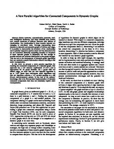
Actual ⌈2 log d⌉

10

5

Max intermediate size

Analysis of Hash-to-Min on a path graph with random node orderings

Number of iterations

Fig. 1.

10 15 20 25 30 35 40

100000

Actual 3(|V | + |E|)

1000 100 1000

d (a) # of Iterations (max over 10 runs) Fig. 2.

100000

100000

|V | + |E|

(b) Largest intermediate data size (average 10 runs)

Analysis of Hash-to-Min on a tree graph with random node orderings

different source, hence the sizes of connected components vary. The number of nodes |V | = 431, 221 (nearly 430K) and the number of edges |E| = 889, 205 (nearly 890K). We also have a sample of this graph (238K nodes and 459K edges) with weighted edges, denoted MovieW, which we use for agglomerative clustering experiments. • Biz: The biz dataset has business listings coming from two overlapping feeds that are licensed by a large internet company. Again edges between two businesses correspond to business listings that are duplicates of one another. Here, |V | = 10, 802, 777 (nearly 10.8M) and |E| = 10, 197, 043 (nearly 10.2M). We also have a version of this graph with weighted edges, denoted BizW, which we use for agglomerative clustering experiments. • Social: The Social dataset has social network edges between users of a large internet company. Social has |V | = 58552777 (nearly 58M) and |E| = 156355406 (nearly 156M). Since social network graphs have low diameter, we remove a random sample of edges, and generate SocialSparse. With |E|= 15, 638, 853 (nearly 15M), SocialSparse graph is more sparse, but has much higher diameter than Social. • Twitter: The Twitter dataset (collected by Cha et al [3]) has follower relationship between twitter users. Twitter has |V | = 42069704 (nearly 42M) and |E| = 1423194279 (nearly 1423M). Again we remove a random sample of

edges, and generate a more sparse graph, TwitterSparse, with |E|= 142308452 (nearly 142M). • Synth: We also synthetically generate graphs of a varying diameter and sizes in order to better understand the properties of the algorithms. A. Connected Components Algorithms: We compare Hash-Min, Hash-Greater-to-Min, Hash-to-All, Hash-to-Min and its load-balanced version Hash-to-Min∗ (Section IV). For Hash-Min, we use the opensource Pegasus implementation8, which has several optimizations over the Hash-Min algorithm. We implemented all other algorithms in Pig9 on Hadoop10. There is no native support for iterative computation on Pig or Hadoop map-reduce. We implement one iteration of our algorithm in Pig and drive a loop using a python script. Implementing the algorithms on iterative map-reduce platforms like HaLoop [2] and Twister [7] is an interesting avenue for future work. 1) Analyzing Hash-to-Min on Synthetic Data: We start by experimentally analyzing the rounds complexity and space requirements of Hash-to-Min. We run it on two kinds of synthetic graphs: paths and complete binary trees. We use synthetic data for this experiment so that we have explicit 8 http://www.cs.cmu.edu/∼ pegasus/ 9 http://pig.apache.org/ 10 http://hadoop.apache.org

10

Fig. 3.

(a) Group I:Runtimes (in minutes)

(b) Group I: # of Map-Reduce jobs

(c) Group II: Runtimes (in minutes)

(d) Group II: # of Map-Reduce jobs

Comparison of Pegasus and our algorithms on real datasets.

control over parameters d, |V |, and |E|. Later we report the performance of Hash-to-Min on real data as well. We use path graphs since they have largest d for a given |V | and complete binary trees since they give a very small d = log |V |. For measuring space requirement, we measure the largest intermediate data size in any iteration of Hash-to-Min. Since the performance of Hash-to-Min depends on the random ordering of the nodes chosen, we choose 10 different random orderings for each input. For number of iterations, we report the worst-case among runs on all random orderings, while for intermediates data size we average the maximum intermediate data size over all runs of Hash-to-Min. This is to verify our conjecture that number of iterations is 2 log d in the worstcase (independent of node ordering) and intermediate space complexity is O(|V | + |E|) in expectation (over possible node orderings). For path graphs, we vary the number of nodes from 32 (25 ) to 524, 288 (219 ). In Figure 1(a), we plot the number of

iterations (worst-case over 10 runs on random orderings) with respect to log d. Since the diameter of a path graph is equal to number of nodes, d varies from 32 to 524, 288 as well. As conjectured the plot is linear and always lies below the line corresponding to 2 log d. In Figure 1(b), we plot the largest intermediate data size (averaged over 10 runs on random orderings) with respect to |V | + |E|. Note that both x-axis and y-axis are in log-scale. Again as conjectured, the plot is linear and always lies below 3(|V | + |E|). For complete binary trees, we again vary the number of nodes from 32 (25 ) to 524, 288 (219 ). The main difference from the path case is that for a complete binary tree, diameter is 2 log(|V |) and hence the diameter varies only from 10 to 38. Again in Figure 2(a), we see that the rounds complexity still lies below the curve for 2 log d supporting our conjecture even for trees. In Figure 2(b), we again see that space complexity grows linearly and is bounded by 3(|V | + |E|).

11

Input Biz Movie SocialSparse

|V |

|E|

10.8M 430K 58M

10.1M 890K 15M

n 93 17K 2.9M

Pegasus # MR jobs 36 60 60

Time 40 263 173

Hash-to-Min # MR jobs Time 7 29 7 17 11 59

Hash-Greater-to-Min # MR jobs Time 23 34 23 59 38 144

Hash-to-All # MR jobs Time 4 14 DNF DNF DNF DNF

TABLE IV C OMPARISON OF P EGASUS , H ASH - TO -M IN , H ASH -G REATER - TO -M IN , AND H ASH - TO -A LL ON THE G ROUP I DATASETS . T IME IS AVERAGED OVER 4 RUNS AND ROUNDED TO MINUTES . O PTIMAL TIMES APPEAR IN BOLD : IN ALL CASES EITHER H ASH - TO -M IN OR H ASH - TO -A LL IS OPTIMAL .

Input Social TwitterSparse Twitter

|V | 58M 42M 42M

|E| 156M 142M 1423M

n 36M 24M 42M

Pegasus # MR jobs 20 12 12

Time 145 57 61

Hash-to-Min∗ # MR jobs Time 7 65 5 32 5 50

TABLE V C OMPARISON OF P EGASUS AND THE H ASH - TO -M IN∗ ALGORITHM ON G ROUP II DATASETS . T IME IS AVERAGED OVER 4 RUNS AND ROUNDED TO MINUTES . O PTIMAL TIMES APPEAR IN BOLD : IN ALL CASES , H M∗ IS OPTIMAL .

Fig. 4.

(a) Runtimes (in minutes) (b) # of Map-Reduce jobs Comparison of Hash-to-All and Hash-to-Min for single linkage clustering on BizW and MovieW.

2) Analysis on Real Data: We next compared Hash-toMin, Hash-Greater-to-Min, and Hash-to-All algorithms on real datasets against Pegasus [10]. To the best of our knowledge, Pegasus is the fastest technique on MapReduce for computing connected components. Although all datasets are sparse (have average degree less than 3), each dataset has very different distribution on the size n of the largest connected components and graph diameter d. We partition our datasets into two groups – group I with d >= 20 and relatively small n, and group II with d < 20 and very large n. Group I: Graphs with large d and small n: This group includes Biz, Movie, and SocialSparse datasets that have large diameters ranging from 20 to 80. On account of large diameters, these graphs requires more MR jobs and hence longer time, even though they are somewhat smaller than the graphs in the other group. These graphs have small connected components that fit in memory. Each connected component in the Biz dataset represents the number of duplicates of a real-world entity. Since there are only two feeds creating this dataset, and each of the two feeds is almost void of duplicates, the size of most connected components is 2. In some extreme cases, there are more duplicates, and the largest connected component we saw had size 93. The Movie dataset has more number of sources,

and consequently significantly more number of duplicates. Hence the size of some of the connected components for it is significantly larger, with the largest containing 17,213 nodes. Finally, the SocialSparse dataset has the largest connected component in this group, with the largest having 2,945,644 nodes. Table IV summarizes the input graph parameters. It also includes the number of map-reduce jobs and the total runtime for all of the four techniques. Differences in the connected component sizes has a very interesting effect on the run-times of the algorithm as shown in Figures 3(a) and 3(b). On account of the extremely small size of connected components, runtime for all algorithms is fastest for the Biz dataset, even though the number of nodes and edges in Biz is larger than the Movie dataset. Hash-to-All has the best performance for this dataset, almost 3 times faster than Pegasus. This is to be expected as Hash-to-All just takes 4 iterations (in general it takes log d iterations) to converge. Since connected components are small, the replication of components, and the large intermediate data size does not affect its performance that much. We believe that Hash-to-All is the fastest algorithm whenever the intermediate data size is not a bottleneck. Hash-to-Min takes twice as many iterations (2 log d in general) and hence takes almost twice the time. Finally, Pegasus takes even more time because of a larger

12

k 1 5 10 15

MR -k Completion Time maximum median 10:45 10:45 17:03 11:30 19:10 12:46 28:17 26:07

BSP-k Completion Time maximum median 7:40 7:40 11:20 8:05 23:39 15:49 64:51 43:37

TABLE VI M EDIAN AND MAXIMUM COMPLETION TIMES ( IN MIN : SEC ) FOR k CONNECTED COMPONENT JOBS DEPLOYED SIMULTANEOUSLY USING MAP - REDUCE ( MR - K ) AND G IRAPH ( BSP - K )

number of iterations, and a larger number of map-reduce jobs. For the Movie and SocialSparse datasets, connected components are much larger. Hence Hash-to-All does not finish on this dataset due to large intermediate data sizes. However, Hash-to-Min beats Pegasus by a factor of nearly 3 in the SocialSparse dataset since it requires a fewer number of iterations. On movies, the difference is the most stark: Hashto-Min has 15 times faster runtime than Pegasus again due to significant difference in the number of iterations. Group II: Graphs with small d and large n: This group includes Social, TwitterSparse, and Twitter dataset that have a small diameter of less than 20, and results are shown in Figures 3(c) and 3(d) and Table V. Unlike Group I, these datasets have very large connected components, such that even a single connected component does not fit into memory of a single mapper. Thus we apply our robust implementation of Hash-to-Min (denoted Hash-to-Min∗ ) described in Sec. IV. The Hash-to-Min∗ algorithm is nearly twice as fast as pegasus, owing to reduction in the number of MR rounds. Only exception is the Twitter graph, where reduction in times is only 18%. This is because the Twitter graph has some nodes with very high degree, which makes load-balancing a problem for all algorithms. B. Single Linkage Clustering We implemented single linkage clustering on map-reduce using both Hash-to-All and Hash-to-Min hashing strategies. We used these algorithms to cluster the MovieW and BizW datasets. Figures 4(a) and 4(b) shows the runtime and number of map-reduce iterations for both these algorithms, respectively. Analogous to our results for connected components, for the MovieW dataset, we find that Hash-to-Min outperforms Hash-to-All both in terms of total time as well as number of rounds. On the BizW dataset, we find that both Hash-toMin and Hash-to-All take exactly the same number of rounds. Nevertheless, Hash-to-All takes lesser time to complete that Hash-to-Min. This is because some clusters (with small n) finish much earlier in Hash-to-All; finished clusters reduce the amount of communication required in further iterations. C. Comparison to Bulk Synchronous Parallel Algorithms Bulk synchronous parallel (BSP) paradigm is generally considered more efficient for graph processing than map-reduce as it has less setup and overhead costs for each new iteration. While the algorithmic improvements of reducing number of iterations presented in this paper are important independent of the underlying system used, these improvements are of less significance in BSP due to low overhead of additional iterations.

In this section, we show that BSP does not necessarily dominate Map-Reduce for large-scale graph processing (and thus our algorithmic improvements for Map-Reduce are still relevant and important). We show this by running an interesting experiment in shared grids having congested environments. We took the Movie graph and computed connected components using Hash-to-Min (map-reduce, with 50 reducers) and using Hash-Min11 on Giraph [4] (BSP, with 100 mappers), an open source implementation of Pregel [16] for Hadoop. We deployed k = 1, 5, 10, and 15 copies of each algorithm (denoted by MR-k and BSP-k), and tracked the maximum and median completion times of the jobs. The jobs were deployed on a shared Hadoop cluster with 454 map slots and 151 reduce slots, and the cluster experienced normal and equal load from other unrelated tasks. Table VI summarizes our results. As expected, BSP-1 outperforms MR-1;12 unlike map-reduce, the BSP paradigm does not have the per-iteration overheads. However, as k increases from 1 to 15, we can see that the maximum and median completion times for jobs increases at a faster rate for BSP-k than for MR-k. This is because the BSP implementation needs to hold all 100 mappers till the job completes. On the other hand, the map-reduce implementation can naturally parallelize the map and reduce rounds of different jobs, thus eliminating the impact of per round overheads. So it is not surprising that while all jobs in MR-15 completed in about 20 minutes, it took an hour for jobs in BSP-15 to complete. Note that the cluster configurations favor BSP implementations since the reducer capacity (which limits the map-reduce implementation of Hash-to-Min) is much smaller (< 34%) than the mapper capacity (which limits the BSP implementation of Hash-Min). We also ran the experiments on clusters with higher ratios of reducers to mappers, and we observe similar results (not included due to space constraints) showing that map-reduce handles congestion better than BSP implementations. VII. C ONCLUSIONS

AND

F UTURE W ORK

In this paper we considered the problem of find connected components in a large graph. We proposed the first mapreduce algorithms that can find the connected components in logarithmic number of iterations – (i) Hash-Greater-toMin, which provably requires at most 3 log n iterations with high probability, and at most 2(|V | + |E|) communication per iteration, and (ii) Hash-to-Min, which has a worse theoretical complexity, but in practice completes in at most 2 log d iterations and 3(|V | + |E|) communication per iteration; n is the size of the largest component and d is the diameter of the graph. We showed how to extend our techniques to the problem of single linkage clustering, and proposed the first algorithm that computes a clustering in provably O(log n) iterations. R EFERENCES [1] F. N. Afrati, V. Borkar, M. Carey, N. Polyzotis, and J. D. Ullman. Mapreduce extensions and recursive queries. In EDBT, 2011. 11 Hash-Min is used as it is easier to implement and not much different than Hash-to-Min in terms of runtime for BSP environment 12 The time taken for MR -1 is different in Tables IV and VI since they were run on different clusters with different number of reducers (100 and 50 resp.).

13

[2] Y. Bu, B. Howe, M. Balazinska, and M. D. Ernst. Haloop: Efficient iterative data processing on large clusters. In VLDB, 2010. [3] M. Cha, H. Haddadi, F. Benevenutoz, and K. P. Gummadi. Measuring user influence in twitter: The million follower fallacy. In ICWSM, 2010. [4] A. Ching and C. Kunz. Giraph : Large-scale graph processing on hadoop. In Hadoop Summit, 2010. [5] J. Cohen. Graph Twiddling in a MapReduce World. Computing in Science and Engineering, 11(4):29–41, July 2009. [6] J. Dean and S. Ghemawat. Mapreduce: simplified data processing on large clusters. Commun. ACM, 51, January 2008. [7] J. Ekanayake, H. Li, B. Zhang, T. Gunarathne, S.-H. Bae, J. Qiu, and G. Fox. Twister: A runtime for iterative mapreduce. In MAPREDUCE, 2010. [8] H. Gazit. An optimal randomized parallel algorithm for finding connected components in a graph. SIAM J. Comput., 20(6):1046–1067, 1991. [9] D. B. Johnson and P. Metaxas. Connected components in o(log3/2n) parallel time for the crew pram. J. Comput. Syst. Sci., 54(2):227–242, 1997. [10] U. Kang, C. E. Tsourakakis, and C. Faloutsos. PEGASUS: A Peta-Scale Graph Mining System- Implementation and Observations. 2009. [11] D. R. Karger, N. Nisan, and M. Parnas. Fast connected components algorithms for the erew pram. SIAM J. Comput., 28(3):1021–1034, 1999.

[12] H. J. Karloff, S. Suri, and S. Vassilvitskii. A model of computation for mapreduce. In SODA, 2010. [13] A. Krishnamurthy, S. S. Lumetta, D. E. Culler, and K. Yelick. Connected components on distributed memory machines. In Parallel Algorithms: 3rd DIMACS Implementation Challenge, 1994. [14] H. R. Lewis and C. H. Papadimitriou. Symmetric space-bounded computation. Theor. Comput. Sci., 19:161–187, 1982. [15] J. Lin and C. Dyer. Data-Intensive Text Processing with MapReduce. Morgan & Claypool Publishers, 2010. [16] G. Malewicz, M. H. Austern, A. J. Bik, J. C. Dehnert, I. Horn, N. Leiser, and G. Czajkowski. Pregel: a system for large-scale graph processing. In SIGMOD, 2010. [17] S. J. Plimpton and K. D. Devine. MapReduce in MPI for Large-scale Graph Algorithms. Special issue of Parallel Computing, 2011. [18] J. Reif. Optimal parallel algorithms for interger sorting and graph connectivity. In Technical report, 1985. [19] T. Seidl, B. Boden, and S. Fries. CC-MR - finding connected components in huge graphs with mapreduce. In ECML/PKDD (1), 2012. [20] Y. Shiloach and U. Vishkin. An O( log n ) parallel connectivity algorithm. Journal of Algorithms, 3:57–67, 1982.

A PPENDIX

14

A. Proof of Theorem 3.6 We first restate Theorem 3.6 below. Theorem A.1 (3.6): Let G = (V, E) be a path graph (i.e. a tree with only nodes of degree 2 or 1). Then, Hash-to-Min correctly computes the connected component of G = (V, E) in 4 log n map-reduce rounds. To prove the above theorem, we first consider path graphs when node ids increase from left to right. Then we show the result for path graphs with arbitrary ordering. Lemma A.2: Consider a path with node ids increasing from the left to right. Then after k iterations of the Hash-to-min algorithm, k • For every node j within a distance of 2 from the minimum node m, m knows j and j knows m. k • For every pair of nodes i, j that are a distance 2 apart, i knows j and j knows k. k • Node j is not known to and does not know any node i that is at a distance > 2 . Proof: The proof is by induction. Base Case: After 1 iterations, each node knows about its 1-hop and 2-hop neighbors (on either side). Induction Hypothesis: Suppose the claim holds after k − 1 iterations. Induction Step: In the k th iteration, consider a node j that is at a distance d from the min node m, where 2k−1 < d ≤ 2k . From the induction hypothesis, there is some node i that is 2k−1 away from j that knows j. Since, m is known to i (from induction hypothesis), the Hash-to-min algorithm would send j to m and m to j in the current iteration. Therefore, m knows j and m is known to j. Consider a node j that is > 2k distance from the min node. At the end of the previous iteration, j knew (and was known to) i, and i knew and was known to i′ – where i and i′ are at distance 2k−1 from j and i respectively. Moreover, i did not know any node i′′ smaller than i′ . Therefore, in the current iteration, i sends i′ to j and j to i′ . Therefore, j knows and is known to a node that is 2k distance away. Finally, we can show that a node does not know (and is not known to) any node that is distance > 2k as follows. Node j can only get a smaller node i′ if i′ is a minimum at some node i. Since in the previous step no one knows a node at distance > 2k−1 , j cannot know a node at distance > 2k . Now we extend the proof for arbitrary path graphs. Denote mink (u) the minimum node after k iterations that u knows that also knows u. Also denote ∆(u, v) the distance between node u and v. Definition A.3 (Local Minima): A node v is local minimum if all its neighbors have id larger than v’s id. For a path graph, we define the notion of levels below. Definition A.4 (Levels): Given a path, level 0 consists of all nodes in the path. Level i is then defined recursively as nodes that are local minimum nodes among the nodes at level i − 1, if the level i − 1 nodes are arranged in the order in which they occur in the path. Denote the set of nodes at level i as level(i). Proposition A.5: The number of levels having more than 1 node is at most log n. Proof: The proof follows from the fact that for each level i, no consecutive nodes can be local minimum. Hence |level(i)| ≤ |level(i − 1)/2). Lemma A.6: Consider a path P with three segments P1 , P2 and P3 , where P1 and P3 are arbitrary, and P2 has r + 1 level ℓ nodes l1 , l2 , ...lr , m1 going from left to right. Assume that labels are such that l1 < l2 < . . . < lr . For a node li , denote l(li , k, ℓ) the closest level ℓ node lj from li towards the right such that mink (lj ) > li . Denote T (k, ℓ) and M (k, ℓ) as T (k, ℓ) = minP,li :l(li ,k,ℓ)6=lr ∆(li , l(li , k, ℓ)) and M (k, ℓ) = minP :mink (l1 )>mink−1 (m1 ) or

mink (m1 )>mink−1 (l1 ) ∆(l1 , m1 )

. Then the following is true: 1) T satisfies the following recurrence realtion T (k, ℓ) ≥ min(T (k − 2, ℓ) + min(T (k − 1, ℓ), M (k, ℓ), M (k − 1, ℓ − 1)) 2) M satisfies the following recurrence relation M (k, ℓ) ≥ min(T (k − 2, ℓ), M (k − 1, ℓ − 1)) Proof: Denote by [lt , lu ] the level ℓ nodes between lt and lu , and [lt , lu ) those nodes except for lu . Proof of claim 1: Let ls = l(li , k − 1, ℓ) and let lt be the level ℓ node just to the left of ls . We know by definition of ls = l(li , k − 1, ℓ) that mink−1 (ls ) > li , but for all l ∈ [li , lt ], mink−1 (l) ≤ li . Now there are three cases: 1) mink−1 (lt ) ∈ P3 . Then mink−1 (lt ) ≤ li (from above), and any node l ∈ [lt , lr ] would have mink−1 (l) ∈ P3 ≤ mink−1 (lt ). Hence mink−1 (l) ≤ li for all l ∈ {li , . . . , lr }. Thus l(li , k − 1) = lr . 2) mink−1 (lt ) ∈ / P3 and ∆(li , lt ) ≥ T (k − 1, ℓ). Denote lu = l(lt , k − 1, ℓ). Consider any l ∈ [lt , lu ). Let a = mink−1 (l). Then from the definition of lu = l(lt , k − 1) and since l ∈ [lt , lu ), we know that, a = mink−1 (l) ≤ lt . Now there are two sub-cases:

15

a) For all l ∈ [lt , lu ), a = mink−1 (l) ∈ / P3 ∪ {m1 }. In this case, we show that l(li , k, ℓ) is a level ℓ node in [lu , lr ]. For this we will show that for all l ∈ [lt , lu ) and a = mink−1 (l), mink−1 (a) ≤ li . If a ∈ / P3 ∪ {m1 }, then either (i) a ∈ P1 , in which case a ≤ l1 (otherwise mink−1 (l) would be l1 and not a), and hence obviously mink−1 (a) ≤ li , or (ii) a ∈ P2 but a 6= m1 , and then since a ≤ lt (from above), a ∈ [li , lt ]. Hence mink−1 (a) ≤ li . In other words, after k − 1 iterations, the minimum for any node l ∈ [lt , lu ) is a, which in turn has a minimum b ≤ li . Thus in one Hash-to-Min step, b would become mink (l). Hence after k iterations and for any local minimum l between li and lu , we have mink (l) ≤ li . This shows that l(li , k, ℓ) ∈ [lu , lr ]. Then either lu is lr or the following holds. ∆(li , l(li , k, ℓ)) ≥ ∆(li , lt ) + ∆(lt , lu ) ≥ T (k − 2, ℓ) + T (k − 1, ℓ − 1) b) There exists l ∈ [lt , lu ), such that a = mink−1 (l) ∈ P3 . Let lw = l(li , k, ℓ). Then lw is the first node in [li , lr ] for which mink (lw ) > li . If ∆(lv , lw ) ≤ M (k, ℓ) then by definition after k iterations mink (lw ) ≤ mink−1 (lt ) ≤ li . Thus ∆(lw , li ) ≥ M (k, ℓ). Thus ∆(li , l(li , k, ℓ)) ≥ ∆(li , lt ) + ∆(lt , lw ) ≥ T (k − 2, ℓ) + M (k, ℓ) 3) mink−1 (lt ) ∈ P1 ||P2 and ∆(li , lt ) ≤ T (k − 2, ℓ). In this case, we argue that ∆(lt , ls ) > M (k − 1, ℓ − 1). Assume the contrary: ∆(lt , ls ) ≤ M (k − 2, ℓ − 1). Since, ∆(li , lt ) ≤ T (k − 2, ℓ), we know that mink−2 (lt ) ≤ li . Since lt and ls are consecutive level ℓ nodes, all the level ℓ − 1 nodes between them are ordered. Hence by definition of M (k − 1, ℓ − 1), and the fact that ∆(lt , ls ) ≤ M (k − 1, ℓ − 1), mink−1 (ls ) ≤ mink−2 (lt ) ≤ li . This contradicts the assumption that ls = l(li , k − 1, ℓ). Thus ∆(lt , ls ) > M (k − 1, ℓ − 1). ∆(li , l(li , k)) ≥ ∆(li , lt ) + ∆(lt , ls ) ≥ M (k − 1, ℓ − 1) Combining the above cases we complete the proof of claim 1. Proof of claim 2: If ∆(l1 , lr ) ≤ T (k−2, ℓ), then mink−2 (lr ) ≤ l1 . Also if ∆(lr , m1 ) ≤ M (k−1, ℓ−1), then mink−1 (m1 ) ≤ mink−2 (lr ) ≤ l1 . If both ∆(l1, lr ) ≤ T (k − 2, ℓ) and ∆(lr , m1 ) ≤ M (k − 1, ℓ − 1), then mink−1 (m1 ) ≤ l1 . Hence by claim 1, mink (m) ≤ mink−1 (l1 ). This completes the proof. Lemma A.7: Let T (k, ℓ) be the quantity as defined in Lemma A.6. Then T (k, ℓ) ≥ 2k/2−ℓ . Proof: We prove the lemma using induction. Base Cases: (i) ℓ = 0 and k ≥ 1. Then by Lemma A.2, T (k, 0) ≥ 2k ≥ 2k/2−0 . (ii) k = 1 and ℓ ≥ 1. For any level ℓ ≥ 1, T (1, ℓ) ≥ 1 ≥ 21/2−ℓ . Induction Hypothesis (IH) For all k0 ≤ k − 1 and ℓ0 ≤ ℓ − 1, T (k0 , ℓ0 ) ≥ 2k0 /2−ℓ0 Induction Step: By Lemma A.6, we know that: T (k, ℓ) ≥ min (T (k − 1, ℓ) + T (k − 2, ℓ), T (k − 2, ℓ − 1))   (using IH) ≥ min 2(k−1)/2−ℓ + 2(k−2)−ℓ , 2(k−2)/2−ℓ+1   √ ≥ min 2k/2−ℓ (1/2 + 1/ 2), 2k/2−ℓ ≥ 2k/2−ℓ

Finally, we can complete the proof of Theorem 3.6. Since T (k, l) is less than the length of the path, we know that T (k, l) < n. Now from Prop. A.5, the number of levels having more than 1 node is at most log n. Hence ℓ ≤ log n. Finally, from Lemma A.7, we know that T (k, ℓ) ≥ 2k/2−ℓ . Thus 2k/2−log n ≤ 2k/2−ℓ ≤ n. Thus k ≤ 4 log n. This completes the proof of Theorem 3.6. B. Proof of Theorem 3.9 We first restate Theorem 3.9 below. Theorem A.8 (3.9): Algorithm Hash-Greater-to-Min correctly computes the connected components of G = (V, E) in expected 3 log n map-reduce rounds (expectation is over the random choices of the node ordering) with 2(|V | + |E|) communication per round in the worst case. Proof: After 3k rounds, denote Mk = {min(Cv ) : v ∈ V } the set of nodes that appear as minimum on some node. For a minimum node m ∈ Mk , denote GTk (m) the set of all nodes v for which m = min(Cv ). Then by Lemma 3.8, we know that GTk (m) = C≥( m) after 3k rounds. Obviously ∪m∈Mk GTk (m) = V and for any m, m′ ∈ Mk , GTk (m) ∩ GTk (m′ ) = ∅. Consider the graph GMk with nodes as Mk and an edge between m ∈ Mk to m′ ∈ Mk if there exists v ∈ GTk (m) and v ′ ∈ GTk (m′ ) such that v, v ′ are neighbors in the input graph G. If a node m has no outgoing edges in GMk , then GTk (m) forms a connected component in G disconnected from other components, this is because, then for all v ′ ∈ / GTk (m), there exists no edge to v ∈ GTk (m).

16

We can safely ignore such sets GTk (m). Let M Ck be the set of nodes in GMk that have at least one outgoing edge. Also if m ∈ M Ck has an edge to m′ < m in GMk , then m will no longer be the minimum of nodes v ∈ GTk (m) after 3 additional rounds. This is because there exist nodes v ∈ GTk (m) and v ′ ∈ GTk (m′ ), such that v and v ′ are neighbors in G. Hence in the first round of Hash-Min, v ′ will send m′ to v. In the second round of Hash-Min, v will send m′ to m. Hence finally m will get m′ , and in the round of Hash-Greater-to-Min, m will send GTk (m) to m′ . If |M Ck | = l, W.L.O.G, we can assume that they are labeled 1, 2, . . . , l (since only relative ordering between them matters anyway). For any set, GTk (m), the probability that it its min m′ ∈ (l/2, l] after 3 more rounds is 1/4. This is because that happens only when m ∈ [(l/2, l) and all its neighbors m′ ∈ GMk are also in (l/2, l]. Since there exist at least one neighbor m′ , the probability of m′ ∈ (l/2, l] is at most 1/2. Hence the probability of any node v having a min m′ ∈ (l/2, l] after 3 more rounds is 1/4. Now since no set, GTk (m), ever get splits in subsequent rounds, the expected number of cores is 3l/4 after 3 more rounds. Hence in three rounds of Hash-Greater-to-Min, the expected number of cores reduces from l to 3l/4, and therefore it will terminate in expected 3 log n time. P The communication complexity is 2(|V |+|E|) per round in the worst-case since the total size of clusters is v C≥v = 2(|V |). C. Proof of Theorem 5.6 We first restate Theorem 5.6 below. Theorem A.9 (5.6): The distributed Algorithm 3 simulates the centralized Algorithm 2, i.e., it outputs the same clustering as Algorithm 2. Proof: Let Ccentral be the clustering output by Algorithm 2. Let Cdistributed be the clustering output by Algorithm 3. We show the result in two parts. First, for any cluster Cdistributed ∈ Cdistributed , there exists a cluster Ccentral ∈ Ccentral such that Cdistributed ⊆ Ccentral . Since Algorithm 3 uses the splitting algorithm 6, it outputs only cores having cluster splits Cl , Cr for which Stoplocal (Cl ) and Stoplocal (Cr ) equal false. Thus we can invoke Lemma 5.5 on Cdistributed to prove that Cdistributed is valid, and the existence of Ccentral such that Cdistributed ⊆ Ccentral . Having shown that Cdistributed ⊆ Ccentral , we now show that, in fact, Cdistributed = Ccentral . Assume the contrary, i.e. Cdistributed ⊂ Ccentral . Since Cdistributed is valid, even the centralized algorithm constructed Cdistributed some time during ′ its execution, and then merged it with some other cluster, say Ccentral . Since Cdistributed is in the output of Algorithm 3, then three cases are pospsible: (i) Cdistributed forms a connected component by itself, disconnected from the rest of the graph, or (ii) Stoplocal (Cdistributed ) is true, and the algorithm stops because ′ of the stopping condition, or (iii) Stoplocal (Cdistributed ) is false, but it merges with some cluster Cdistributed for which ′ Stoplocal (Cdistributed ) is true. In the first two cases, even the centralized algorithm can not merge Cdistributed with any other cluster, contradicting that Cdistributed ⊂ Ccentral . ′ ′ ′ ⊆ Ccentral . Since the central algorithm merges Ccentral with Ccentral , For case (iii), we show below that in fact Cdistributed ′ ′ ′ ′ Stoplocal (Ccentral ) has to be false. Since Stoplocal is monotonic, and Cdistributed ⊆ Ccentral , Stoplocal (Cdistributed ) has to be false as well, contradicting the assumption made in case (iii). Thus we proved all three cases are impossible, contradicting our assumption of Cdistributed ⊂ Ccentral . Hence Cdistributed = Ccentral . ′ ′ ′ ′ Now we show that Cdistributed ⊆ Ccentral . Both Cdistributed and Ccentral have to be closest to Cdistributed , i.e. in nbrs(Cdistributed ), in order to get merged with it in either the central or distributed algorithms. Denote v to be the node, such ′ that the singleton cluster {v} is in nbrs(Cdistributed ). Hence, by the property of single linkage clustering, both Cdistributed ′ ′ and Ccentral must contain the node v. Since Cdistributed is valid, there must be a cluster in the central algorithm’s output ′ ′ containing it. Finally, since clusters in the output have to be disjoint, the cluster containing Cdistributed has to be Ccentral , ′ ′ and thus Cdistributed ⊆ Ccentral .