temporal pattern mining process is a large longitudinal patient database collected as ... retinopathy application, the data warehousing and cleaning process, and.
Finding Temporal Patterns in Noisy Longitudinal Data: A Study in Diabetic Retinopathy Vassiliki Somaraki1,2 , Deborah Broadbent2.3 , Frans Coenen1 , Simon Harding2,3 1
Dept. of Computer Science, The University of Liverpool, Liverpool L69 3BX, UK 2 Ophthamology Research Unit, School. of Clinical Science, The University of Liverpool, Liverpool L69 3GA, UK 3 St. Pauls Eye Unit, Royal Liverpool University Hospital, L7 8XP, UK {V.Somaraki,D.M.Broadbent,coenen,sharding}@liverpool.ac.uk
Abstract. This paper describes an approach to temporal pattern mining using the concept of user defined temporal prototypes to define the nature of the trends of interests. The temporal patterns are defined in terms of sequences of support values associated with identified frequent patterns. The prototypes are defined mathematically so that they can be mapped onto the temporal patterns. The focus for the advocated temporal pattern mining process is a large longitudinal patient database collected as part of a diabetic retinopathy screening programme, The data set is, in itself, also of interest as it is very noisy (in common with other similar medical datasets) and does not feature a clear association between specific time stamps and subsets of the data. The diabetic retinopathy application, the data warehousing and cleaning process, and the frequent pattern mining procedure (together with the application of the prototype concept) are all described in the paper. An evaluation of the frequent pattern mining process is also presented. Keywords: Temporal Pattern Mining, Trend Mining.
1
Introduction
This paper describes an approach to finding temporal patterns in noisy longitudinal patient data. The identification of patterns in such data has many applications. One common example is the analysis of questionnaire returns collated over a number of years, for example Kimm et al. studied the nature of physical activity in groups of adolescents ([9]) and Skinner et al. studied children’s food eating habits ([15]). Another example of the application of longitudinal studies is in the analysis of statistical trends; an early reported example is that of Wagner et al. [17], who performed an extensive longitudinal study of children with “special educational needs”. Longitudinal studies particularly lend themselves to the analysis of patient data in medical environments where records of a series of “consultations” are available. For example Yamaguchi et al. ([18]) studied the effect of treatments for shoulder injuries, and Levy et al. [10] studied the
long term effects of Alzheimer’s disease. The application domain, with respect to this paper, is the longitudinal diabetic retinopathy screening data collected by The Royal Liverpool University Hospital (RLUH), a major centre for retinopathy research. The nature of the longitudinal data is of interest because it does not fit into any standard categorisation of such data, in that the “time stamp” used is the sequential patient consultation event number. The duration between consultations is also variable. The temporal patterns of interest, in the context of this paper are frequent patterns (collections of attributes that appear together regularly) that feature some prescribed change in their frequency between two or more time stamps (i.e. a trend). For example patterns whose frequency increases/decreases overtime, patterns whose frequency remains constant with time, or patterns that display some other kind of trend. The patterns themselves are identified using a modified frequent pattern mining algorithm: the TFP algorithm [2, 3] is used in this study, however alternative frequent pattern miners could be suitably modified. The proposed temporal pattern mining process is described in detail. A further challenge of the work described is that the data collection is extremely large and complex; 150,000 records, comprising some 450 fields (of various types: categorical, quantitative, text, etc.), distributed over two databases each composed of a number of tables. The main challenge represented by the data was that, unlike more standard longitudinal data sets, there was no clear association between specific time stamps and subsets of the data. The data warehousing process established to prepare the data for mining is therefore also described. A further complication was that the data, in common with similar patient data sets, was very “noisy” in that it contained many missing and anomalous data. This issue was addressed by defining a set of logic rules. In the context of missing data the logic rules were used to derive appropriate values. In the case of anomalous data the logic rules were used to derive additional fields to formulate “consensus values”. The data cleaning and warehousing process is also described in detail. The principal contributions made by this paper may be summarised as follows: 1. A process for identifying temporal patterns in large longitudinal data sets over a sequence of time stamps. 2. An illustration of the application of the technique to a “real life” data set (including the data cleaning process required to facilitate this illustration). 3. The use of logic rules to address the joint issues of missing and anomalous data. The rest of this paper is organised as follows. Further detail of the retinopathy application domain is given in Section 2. Some background with respect to longitudinal data mining, the concept of temporal pattern mining and the issue of missing values in data is given in Section 3. The adopted data warehousing and cleaning process is described in Section 4. The temporal pattern mining problem and its resolution is described in 5. An evaluation of the process is pre-
sented in Section 6. A summary of the work described, the main findings and some closing observations are presented in section 7.
2
Diabetic Retinopathy Screening
The Royal Liverpool University Hospital (RLUH) has been a major centre for retinopathy research since 1991. Retinopathy is a generic term used to describe damage to the retina of the eye which can, in the long term, lead to visual loss. Retinopathy can result from a number of causes, for example: diabetes, agerelated macular degeneration (AMD), high blood pressure and various genetic conditions. In diabetes the retinopathy progresses over a number of years through well characterised stages. Treatment comprises the application of laser to the retina and is most effective during the stages before vision is affected. Screening programmes for people with diabetes have recently been established across the UK to detect retinopathy and instigate prompt treatment. RLUH has collected a substantial amount of data, over a considerable period, of time as part of its diabetic retinopathy research and screening programme. Screening takes place within the community and is conducted by technicians who perform photography and record data images on “lap-tops” which are then downloaded (typically) at the end of each day. Retinal images are graded at a central grading facility at a separate time, but within a few weeks, with results recorded into a database. If the level of disease detected in the retinal photographs is worse than a predetermined level, or if photographs are ungradable or unobtainable, then screenees are invited to a dedicated hospital outpatient clinic for further examination by an ophthalmologist using more specialised slit lamp biomicroscopy1 . Data on retinal findings are entered into the database. This clinical assessment can occur several months after the initial photographic screening. Four types of data associated with a single screening sequence are collected: 1. 2. 3. 4.
General demographic data. Data on visual acuity (clarity of vision). Data from grading of retinal images. Data from biomicroscopy of the retina.
The full screening sequence is referred to as a “screening episode” People with diabetes are usually screened once a year with the option to rescreen early (typically 6 months) depending on the presence of intermediate levels of disease indicating greater risk of progression. The RLUH screening programme currently deals with some 17,000 people with diabetes registered with family doctors within the Liverpool Primary Care Trust2 per year. Overall details of some 20,000 patients have been recorded. Consequently a substantial amount of data is available for analysis. Some further details of the data collection are presented in the following sub-section. 1 2
A high intensity light source instrument to facilitate examination of the human eye. A Primary Care Trusts (PCTs) are organisational units established to manage local health services in the UK.
2.1
Data Storage
Data collected from the diabetic retinopathy screening process described above is stored in a number of databases. The structure (tables) of these database reflect the mechanism whereby patients are processed and includes historical changes in the process. Screening commenced in 1991 when data was recorded in a bespoke database system called Epi-Info. Epi-Info was replaced with a more sophisticated system, Diabolos, in 1995, which describes the data used in this study. Diabolos, in turn, was replaced with a national database system, Orion, in 2005. The design and implementation of Orion does not lend itself to simple extraction of data for temporal pattern mining purposes and thus the data contained in this latest database system does not form part of the current study. Thus the study described here deals with data collected from 1995 to 2005. The RLUH, as opposed to the screening programme, also maintains a clinical investigations database called ICE. This database includes information about biochemical “risk factors” that are known to be associated with progression of diabetic retinopathy. Not all patients included in the screening programme have records on ICE. The screening programme has its own Risk Factors database, maintained by the programme team, containing data mostly extracted from ICE. In the context of temporal pattern mining there are therefore five tables used in this study of which the first four are held in the Diabolos system: 1. Patient Details. Table containing background information regarding individual patients. 2. General. Demographic patient details and visual acuity data. 3. Photo Details. Results from the photographic grading. 4. Biomicroscopy. Results from the slit lamp biomicroscopy in cases where this has been conducted. 5. Risk Factors. Results from blood pressure and biochemistry investigations known to be associated with an increased risk of progression of retinopathy.
3
Previous Work
This previous work section comprises three subsections, each focussing on one of the three Knowledge Discovery in Data (KDD) research domains encompassed by the work described in this paper: (i) longitudinal data mining, (ii) temporal pattern mining, and (iii) missing and anomalous data. 3.1
Longitudinal Data Mining
Longitudinal data is information comprising values for a set of data fields which are repeatedly collected for the same object over a sequence of sample points, as such it can be said to track the progress of the object in some context. The exemplar longitudinal data set is patient data, where information concerning a patient’s condition is repeatedly collected so as to track the patient’s progress.
Longitudinal data may be categorized in a number of ways, one suggested categorization is that of Singer and Willet [14] who identify person-level and person-period data sets. In a person-level data set each person (subject) has one record and multiple variables containing the data from each sampling. In a person-period data set each person (subject) has multiple records, one for each measurement occasion. Thus person-level data set has as many records as there are subjects in the sample, while a person-period data sets has many more records (one for each subject sampling event). The former is sometimes referred to as a broad data structure and the later as long data structure [16]. Longitudinal studies have variations regarding sample size, number of variables and number of time stamps. Broadly speaking, there are five main types of longitudinal study based on these characteristics [6]: (i) simultaneous crosssectional studies, (ii) trend studies, (iii) times series studies, (iv) intervention studies and (v) panel studies. The work described in this paper may be described as a time series study, in order to identify trends contained in a person-period data set. 3.2
Temporal Pattern Mining
The objective of temporal pattern mining (or trend mining) is to discover temporal patterns in time stamped data. For example Nohuddin et al. [13] investigate the application of trend mining in cattle movement databases. With respect to diabetic retinopathy data the objective of the temporal pattern mining is to identify unexpected, previously unknown, trends in the data. However, the identification of known patterns is also seen as important as this would provide a means of validating the adopted approach. The process of frequent patten mining in static data tables is well established within the Knowledge Discovery in Data (KDD) community and can be traced back to early work on Association Rule Mining (ARM) as first espoused by Agrawal and Srikant [1]. Less attention has been applied to temporal pattern mining. There has been reported work on Temporal ARM (TARM) where association rules are mined from time stamped data. The temporal pattern mining process described in this paper operates on binary value data sets (thus, where necessary, data must be transformed into this format using a process of normalisation and discretisation). The research described in this work also borrows from the field of Jumping and Emerging Patten (JEP) mining as first introduced by Dong and Li ([4]). The distinction between the work on JEPs, and that described in this paper, is that JEPs are patterns whose frequency increases (typically) between two data sets (although some work has been done on identifying JEPs across multiple data sets, for example Khan et al. [8]). JEP mining is usually also conducted in the context of classification (see for example [5]). The distinction between JEPs and the work described here is that the work is directed at pattens that change in a variety of pre-described ways over a sequence of data sets. To the best knowledge of the authors there is little reported work on temporal pattern mining or trend mining as defined above.
Zhu et al. [19], in the context of data stream mining, identify three processing models for temporal pattern mining: (i) Landmark, (ii) Damped and (iii) Sliding Windows. The Landmark model discovers all frequent patterns over the entire history of the data from a particular point in time called the “landmark”. The Damped model, also known as the Time-Fading model, finds frequent patterns in which each time stamp is assigned a weight that decreases with “age” so that older records contribute less than more recent records. In the Sliding Window model the data is mined by sliding a “window” through the temporal dimension. A similar categorisation may be adopted with respect to temporal pattern mining. The work described in this paper adopts the Landmark model. 3.3
Missing and Anomalous Data
The problem of missing attribute values is well established in the context of data mining. The generally agreed view is that removing records with missing data is the least favoured option as this may introduce bias. The reduction of the overall data set size, by removing records that contain missing values, is not considered to be critical. There is significant scientific work to support this view. Approaches to the imputation of missing values has been extensively researched from a statistical perspective [7, 11, 12]. Example imputation methods include: nearest neighbour imputation, mean imputation, ratio imputation and regression imputation. The approach to missing data advocated in this paper is to define and implement a set of logical rules to address the missing value problem, this is discussed further in the following section.
4
Data Warehousing and Cleaning
For the study described in this paper, before any investigation of temporal pattern mining could commence the five database tables identified in Section 2 (Patient, General, Photo Details, Biomicroscopy and Risk factors) were combined into a single warehouse (i.e. a static data repository specifically intended for the application data mining and data analysis tools). The creation of the data warehouse required data anonimisation and data cleaning. The anonimisation of the data tables was initiated by removing patient names. Although this was straightforward, this presented a second problem as in many cases the patient name was the “common key” linking database tables. An obvious candidate for a universal common key was patient NHS (National Health Service) numbers, however this was missing with respect to some 8000 records and consequently had to be added manually. The NHS number was then used for the construction of the data warehouse; on completion the NHS number was replaced by a sequential record number so that individual records could not be traced back to individual patients. The next step after anonimisation was data cleaning. There were three principal issues to be addressed: 1. Missing values.
2. Contradictory values. 3. Duplicate records. The first two issues were addressed by developing a set of logic rules. With respect to missing values the evidence of such a missing value could be interpreted in two ways: (i) that the value was either unknown or mistakenly omitted at time of collection, or (ii) the missing value indicated a negative response to a question suggested by the field, or (iii) the clinician considered the field to be inapplicable for the given case. For example some fields indicated responses to question such as “does the patient have one eye”, to which, in many cases, the clinician had inserted a “yes” if the answer to the question was an affirmative and left the field blank otherwise (the latter can thus be interpreted as either a “no”, or a “don’t know”). A set of “if . . . then . . . ” logical rules were therefore developed to address this issue. The logic rules were written in such a way that they could also be used for data validation purposes. The operation of these rules is best illustrated using some examples. Consider the field SeeGP Regularly 3 featured in the Diabolos General Table. This field can have three possible values: 1 (“No”), 2 (”Yes”) and 9 (“Don’t know”). In the event of a missing value for this field may be derived from another field, in the set of database tables, LastSeeGP ; asking when the patient last saw their GP for anything. The LastSeeGP field can have the following values: 1 (“Within last 6 months”), 2 (“Within last 6 to 12 months”), 3 (“More than a year ago”) and 9 (“Don’t know”). The logic rule is then as shown in Table 1 (the null value indicates a missing field). The rule states that if the value for SeeGP Regularly is missing and the value for LastSeeGP is also missing, or set to 9 (“Don’t know”), we set the value for SeeGP Regularly to 9. If the patient has seen their GP with the last 12 months (LastSeeGP field set to 1 or 2) we set the value for SeeGP Regularly to 2 (“Yes”). Otherwise we set the value of SeeGP Regularly to 1. if (SeeGP Regulary == null) { if (LastSeeGP == 9) or (LastSeeGP == null) then (SeeGP Regulary = 9) if (LastSeeGP == 1) or (LastSeeGP == 2) then (SeeGP Regulary = 2) if (LastSeeGP == 3) then (SeeGP Regulary = 1) } Table 1. SeeGP Regulary Logic Rule
With respect to contradictory/anomalous values this issue can be exemplified by the diAgeDiag field, the age of the patient when diabetes was first diagnosed. Within the application domain this has been recognised as a question patients find very difficult to answer, and consequently clinicians responsible for gathering data often leave this field blank if they feel that a patient is unable to give a definitive answer. In addition it was found that patients may give a different 3
In the UK GP stands for “General Practitioner”, essentially a family doctor; so the field is asking if the patient sees their doctor regularly.
answer over different consultations which was believed to get less accurate with the passing of time. The rule adopted in this case was to take the first recorded value of the field as this was likely to be the most accurate. The duplicate records issue, only prevalent in the Risk factor table, was addressed by issuing search queries to identify duplicate records and then manually removing the duplicates (a time consuming task). On completion of the anonimisation and data cleaning processes the information contained in the data warehouse comprised comprised 1200 binary valued attributes derived from the 53 fields after normalisation/discretisation. The number of records remained more or less unchanged, at 150,000, each describing a single patient consultation (a small number of corrupted and duplicated records were removed). Longitudinal data sets could then be extracted from this warehouse using various parameters. 4.1
Episodes
From Section 2 the temporal window during which data associated with a single screening is collected, is referred to as an episode. Patients are usually screened once a year although there are many exceptions. For the temporal pattern identification process the annual sequence was taken as the “time stamp”. The number of screening episodes per patient that have been recorded varies (at time of writing) between one and twenty with an average number of five consultations. It should also be noted that in some cases a patient might not participate in an annual screening episode, in which case there was no record for that episode although this did not adversely affect the temporal pattern mining process. In some other cases the sequence of episodes terminated because the patient “dropped” out of the screening programme (was referred into the Hospital Eye Service; moved away; died). The data associated with a single episode, as also noted above, may actually be recorded over several months. In some cases it was not clear whether a particular set of data entries belonged to a single episode or not. Some empirical evaluation indicated that the elapsed time between logging the initial screening data and (where appropriate) the results of biomicroscopy was less than 91 days. This was used as a working threshold to identify episode boundaries. For the research described here a window of 91 days was therefore used to collate data into a single “screening episode”. The time lapse between screening episodes is typically twelve months although the data collection displays a great deal of variation resulting from practical considerations effecting the implementation of the screening programme (this is illustrated in Figure 1. As noted above, according to the nature of the retinopathy, additional episodes may take place. Consequently more than one consultation can take place per year in which case the second consultation was ignored. In summary: – The time stamps used in the temporal patten study are episode numbers.
– The study assumes one episode (consultation) per year; where more than one took place in each time stamp the earliest one was used. – To associate appropriate patient data with a single episode a 90 day window was used. – Where a specific 91 day window included multiple data records, the most recent data (within the window) was used.
Fig. 1. Time lapse between screening (t = number of days between screenings)
4.2
Normalisation and Discretisation
The temporal pattern mining process (see below for further detail) operated using binary valued data only (frequent pattern mining is typically directed at binary value data). Thus the longitudinal data sets extracted from the data warehouse had to be converted in this format. The LUCS-KDD DN pre-processing software4 was used for this process. Continuous values were discretised into prescribed k ranges giving rise to k binary valued (yes/no) attributes for a single field describing continuous data. Categorical valued fields were normalised so that a field that could have k values was described by k attributes (one per value). 4
http://www.csc.liv.ac.uk/˜frans/KDD/Software/LUCS-KDD-DN ARM/lucskdd DN.html.
5
The Temporal Pattern Mining Process
Temporal data comprises a sequence of time stamped data sets. In the context of the work described here a temporal data set comprises a a data set D made up of a sequence of episodes E1 , · · · , En (where n is the number of episodes) and each episode comprises a set of records, E = {R1 , · · · , Rm } (where m is the number of records). The ith record within the jth episode is denoted by Rij ; the sequence of records Ri1 to Rim denote the sequence of records associated with patient i for episode 1 to m. Each record comprises some subset of an identified global set of attributes A which in turn represent the possible fieldvalues that exist in the original data set. The objective is to find patterns that exist across the set of episode (E) that feature specific trends. The pattens are defined in terms of subsets of A that occur frequently within episodes. The temporal patterns (trends) are then defined in terms of the changing support values between adjacent episodes. Thus a temporal pattern is defined as a tuple (a, S) where a is an itemset such that a ⊂ A, and S = {s1 , · · · , sn } such that si is the support for the itemset a at episode i. Trends in temporal patterns are then defined using mathematical identities (prototypes). For example an increasing trend line would be defined as follows. trend =
N −1 X i=1
Si+1 − Si +1 Si
(1)
Thus if {Si+1 }/Si > 1 for all i from i = 1 to i = n − 1, and the trend (Growth Rate) is greater than some user defined Growth Rate Threshold, p, then the associated attribute set is displaying an “increasing” trend. The value of p is selected according to the magnitude of the trend increase that the end user is interested in. Note that this increasing trend concept operates in a similar manner to the Emerging pattern (EP) concept [4], as described above, except that the patterns exist across many data sets whereas JEPs are normally determined with respect to two data sets. The similarity is sufficient to allow operational comparisons to be made as reported in the following section. Decreasing trends and “constant” trends may be defined in a similar manner as follows. If {si+1 }/Si < 1 for all i from i = 1 to i = n − 1, and the trend (Growth Rate) is less than some user defined Growth Rate Threshold, p, then the associated attribute set is displaying a “decreasing” trend. Note that in this case the Growth Rate will be negative. If {si+1 }/Si = 1±k for all i from i = 1 to i = n − 1, and the trend (Growth Rate) is constant (±k), where k is a Tolerance Threshold, then that attribute set is said to be displaying a “constant” trend. The temporal pattens were generated by applying a frequent pattern mining algorithm to each episode in a given longitudinal data set. The Total From Partial (TFP) algorithm [2, 3] was used. TFP is a fast pattern mining algorithm that operates using the support-confidence framework [1]. The support threshold was used to limit the number of potential patterns that might be of interest. Note that for a temporal pattern to be recorded it must be frequent at all time stamps, therefore a low support threshold must be used.
Fig. 2. Number of temporal patterns, increasing trends, identified using the advocated approach
Fig. 3. Number of temporal patterns identified using EP mining (Dong and Li [4])
Fig. 4. Number of constant patterns using different values of k
6
Evaluation
The above temporal pattern mining process was evaluated using a three episode longitudinal data set extracted from the data warehouse (as defined above). Three episodes (E1 , · · · , E3 ) was chosen as this was anticipated to result in a large number of patterns. The data set used comprised 9,400 records. The first experiment reported here compares the operation of the advocated frequent pattern mining approach, in the context of the increasing trends proto-type, with the concept of Emerging Pattern (EP) mining. The comparison is made in terms of the number of temporal patterns (EPs) generated. Recall that JEP mining finds patterns that exist between pairs of data sets; i.e. E1 and E2 , and E2 and E3 in this case: thus two sets of JEPs will be identified with respect to the given data. The results are presented in Figures 5 and 3. The figures indicate the number of discovered patterns using a number of Growth Thresholds (p) from p = 1.1 to p = 1.8 and three support thresholds (s = 0.5, s = 0.05 and s = 0.005). Figure 5 gives the number of patterns produced using the advocated approach, and Figure 3 the number of patterns using standard EP mining. Comparison of the figures indicates that, using the advocated approach, fewer patterns are produced than when adopting EP mining. From the figures it can also be seen that, as the Growth Rate Threshold (p) value is increased, the number of trends (EPs) decreases as only the “steeper” trends are discovered. The figures also confirm that, as expected, the number of identified patterns increases as the user defined support threshold (s) decreases.
The second experiment considered the effect of the value of the Tolerance Threshold, k, on the number of detected constant trends. A range of k values (from 0.005 to 0.055) were used coupled with the sequence of support thresholds used in the previous experiments. The results are presented in Figure 4. From the graph it can be seen that the support threshold setting has a much greater effect on the number of constant trends identified than the value of k. For completeness Table 2 presents a summary of the number of patterns discovered in each category (increasing, decreasing, constant) using a range of support thresholds. With respect to the increasing and decreasing trend patterns a Growth Rate Threshold, p, of 1.1 was used. With respect to the constant patterns a Tolerance Threshold, k, of 0.05. was used. Support T’hold Increasing Decreasing Constant Total 0.005 1559 499 371 2429 0.05 996 378 76 1450 0.5 392 221 38 651 Table 2. Number of Identified Increasing, Decreasing and Constant Patterns (p = 1.1, k = 0.05)
7
Summary and Conclusion
In this paper we have described an approach to temporal patten mining as applied within the context of a diabetic retinopathy application. The particular application was of interest because it comprised a large longitudinal data set that contained a lot of noise and thus presented a significant challenge in several areas. A mechanism for generating specific temporal patterns was described where the nature of the desired patterns is defined using prototypes (which are themselves defined mathematically). The technique was evaluated by considering the effect of changing the threshold values required by the system and comparing with an established Emerging Pattern (EP) mining approach. The paper also describes an interesting approach to data cleaning using the concept of logic rules to address issues of missing values and contradictory/anomalous values. The research team have been greatly encouraged by the results, and are currently working on more versatile mechanisms for defining prototypes, so that a greater variety of prototypes can be specified. For example the specification of a minimum and maximum p threshold. In addition novel techniques for interpretation of output in a clinical setting are being developed.
References 1. Agrawal, R. and Srikant, R. Fast Algorithms for mining Association Rules. Proc. 20th Very Large Data Bases conference (VLDB’94), 487-449 (1994). 2. Coenen, F.P., Leng, P. and Ahmed, S. Data Structures for association Rule Mining: T-trees and P-trees. IEEE Transactions on Data and Knowledge Engineering, 16(6), 774-778 (2004).
3. Coenen, F.P. Leng, P., and Goulbourne, G. Tree Structures for Mining Association Rules. Journal of Data Mining and Knowledge Discovery, 8(1), 25-51 (2004). 4. Dong, G. and Li. J. Efficient Mining of Emerging Patterns: Discovering Trends and Differences. Proc. SIGKDD. ACM, 43-52 (1999). 5. Fan, H. and Kotagiri, R. A Bayesian Approach to Use Emerging Patterns for classification Proceedings of the 14th Australasian database conference, 17, 39-48 (2003). 6. van der Kamp, L.J.T. and Bijleveld, C.C.J.H. Methodological issues in longitudinal research. In: Bijleveld, C.C.J.H., van der Kamp, L.J.T. , Mooijaart, A., van der Kloot, W., van der Leeden, R. and van Der Burg, E., Longitudinal Data Analysis, Designs Models and Methods. SAGE publications, 1-45 (1988). 7. Kalton, G. and Kasprzyk, D. The treatment of missing survey data. Survey Methodology, 12, 1-16 (1986). 8. Khan, M.S., Coenen, F., Reid, D., Tawfik, H., Patel, R. and Lawson, A. A Sliding Windows based Dual Support Framework for Discovering Emerging Trends from Temporal Data. To appear in KBS Journal (2010). 9. Kimm, S.Y.S., Glynn, N.W., Kriska, A.M. Fitzgerald, S. L., Aaron, D. J., Similo, S.L., McMahon, R.P, Barton, B.A. Longitudinal changes in physical activity in a biracial cohort during adolescence. Medicine and Science in Sports and Exercise, 32(8), 1445-1454 (2000). 10. Levy, M.L., Cummings, J.L., Fairbanks, L.A., Bravi, D., Calvani M. and Carta, A. Longitudinal assessment of symptoms of depression, agitation, and psychosis in 181 patients with Alzheimer’s disease. American Journal of Psychiatry, 153, 1438-1443 (1996). 11. Little, R. J. and Rubin, D.B. Statistical Analysis with Missing Data. Second Edition. John Wiley and Sons, New York (2002). 12. Mumoz, ˜ J.F. and Rueda, M. New imputation methods for missing data using quantiles. Journal of Computational and Applied Mathematics, 232(2), 305-317 (2009). 13. Nohuddin, P.N.E., Coenen, F., Christley, R. and Setzkorn, C. Trend Mining in Social Networks: A Study Using A Large Cattle Movement Database. To appear, Proc. ibia Industrial Conf. on Data Mining, Springer, LNAI (2010). 14. Singer, J.D. and Willet, J.B. Applied longitudinal data analysis modelling change and event occurrence. Oxford University Press (2003). 15. Skinner, J.D., Carruth, B.R., Wendy, B. and Ziegler, P.J. Children’s Food Preferences A Longitudinal Analysis. Journal of the American Dietetic Association, 102(11), 1638-1647 (2002). 16. Twisk, J.W.R. Applied longitudinal data analysis for epidemiology: a practical guide. Cambridge University Press (2003). 17. Wagner, M, “and others”. What Happens Next? Trends in Postschool Outcomes of Youth with Disabilities: The Second Comprehensive Report from the National Longitudinal Transition Study of Special Education Students. SRI International, 333 Ravenswood Ave., Menlo Park, CA 94025-3493 (1992). 18. Yamaguchi, K., Tetro, A.M., Blam, O., Evanoff, B.A., Teefey S.A. and Middleton, W.D. Natural history of asymptomatic rotator cuff tears: A longitudinal analysis of asymptomatic tears detected sonographically. Journal of Shoulder and Elbow Surgery, 10(3),199-203 (2001). 19. Zhu, Y. and Shasha, D. StatStream: Statistical Monitoring of Thousands of Data Streams in Real Time. Proc VLDB, 358-369 (2002).