FINITE ELEMENT APPROXIMATION OF THE NON-ISOTHERMAL ...

c 2007 Institute for Scientific ° Computing and Information

INTERNATIONAL JOURNAL OF NUMERICAL ANALYSIS AND MODELING Volume 4, Number 3-4, Pages 425–440

FINITE ELEMENT APPROXIMATION OF THE NON-ISOTHERMAL STOKES-OLDROYD EQUATIONS CHRISTOPHER COX, HYESUK LEE, AND DAVID SZURLEY Dedicated to Max Gunzburger on the occasion of his 60th birthday. Abstract. We consider the Stokes-Oldroyd equations, defined here as the Stokes equations with the Newtonian constitutive equation explicitly included. Thus a polymer-like stress tensor is included so that the dependent variable structure of a viscoelastic model is in place. The energy equation is coupled with the mass, momentum, and constitutive equations through the use of temperature-dependent viscosity terms in both the constitutive model and the momentum equation. Earlier works assumed temperature-dependent constitutive (polymer) and Newtonian (solvent) viscosities when describing the model equations, but made the simplifying assumption of a constant solvent viscosity when carrying out analysis and computations; we assume no such simplification. Our analysis coupled with numerical solution of the problem with both temperature-dependent viscosities distinguishes this work from earlier efforts. Key Words. viscous fluid, non-isothermal, finite elements, Stokes-Oldroyd.

1. Introduction Viscoelastic flows occur in a variety of applications, including polymer processing. The complexity of the governing equations and the physical domains makes analysis of the mathematical models and the associated numerical methods especially difficult. Current efforts to model viscoelastic flows often revolve around the solution of a (modified) Stokes problem, [5]. The isothermal linear elasticity equations, modified in form to have the same dependent variable structure as the equations governing viscoelastic flows, is analyzed along with a numerical solution in [2]. The Stokes problem is a special case (the incompressible limit) of the equations considered in that work. The purpose of this paper is to analyze the finite element solution of the nonisothermal Stokes problem, modified similarly as in [2]. Thermodynamics play a prominent role in many viscoelastic flow scenarios, especially in polymer processing. Realistic models must ultimately include temperature dependence, since flow characteristics such as viscosity vary widely as temperature varies within normal operating constraints, [1]. The rest of this paper is outlined as follows. The governing equations are presented in the next section, with particular attention given to the manner in which temperature dependence is expressed. Details regarding the weak formulation and Received by the editors February 21, 2006 and, in revised form, February 23, 2006. 2000 Mathematics Subject Classification. 65N30. This research was supported in part by the ERC program of the National Science Foundation under Award Number EEC-9731680 through the Center for Advanced Engineering Fibers and Films at Clemson University. 425

426

C. COX, H. LEE, AND D. SZURLEY

corresponding function spaces are provided in Section 3. In Section 4, the finite element formulation is developed along with an existence result for the finite element solution. Convergence results for the finite element solution are derived in Section 5, and numerical confirmation of these results are presented in Section 6. The paper concludes with a summary and a discussion of continuing work. 2. Governing Equations ´

We consider fluid flowing through a bounded, connected domain Ω ⊂ Rd , whose boundary we denote as Γ. Let the velocity be denoted by u, pressure p, extra stress σ, temperature T , and unit outward normal to the boundary n. For viscoelastic fluid flow, the extra stress tensor is often split into a solvent and polymer part, σ = σs + σp . Normally the solvent part of the extra stress is assumed to be Newtonian, i.e. ηs (T ) d(u), σs = 2 η0 (TR ) where the rate-of-deformation tensor d(u) is defined as ´ 1³ T d(u) = ∇u + (∇u) , 2 ηS is the solvent viscosity which depends at most on the temperature, and η0 (TR ) is the zero-shear viscosity at a reference temperature TR . A nonlinear differential or integral constitutive model is imposed for the polymer part σ p , [1]. As in [2], we simplify the constitutive model to a Newtonian relationship, and include this equation explicitly to preserve the dependent variable structure associated with viscoelastic constitutive models, such as Giesekus or Oldroyd-B. Whereas only the isothermal case is considered in [2], we analyze the case where both σ p and σ s depend on temperature. Specifically, we assume that (2.1)

σ p − 2α1 (T )d(u) = 0,

where an Arrhenius equation characterizes the dependence of polymer viscosity (also scaled to η0 (TR )) upon temperature, i.e. µ ¶ B1 α1 (T ) = A1 exp , T and B1 6= 0. The coefficients A1 and B1 are defined so that 0 < α1 (T ) ≤ 1. We assume the existence of maximum and minimum values for the viscosity (2.2)

α1,min ≤ α1 (T ) ≤ α1,max .

The (scaled) solvent viscosity is defined in a similar manner so that (2.3)

σ s − 2²α2 (T )d(u) = 0,

with

µ

¶ B2 . T Once again we choose A2 and B2 so that 0 < α2 (T ) ≤ 1 and α2 (T ) = A2 exp

(2.4)

α2,min ≤ α2 (T ) ≤ α2,max ,

but here we may have B2 = 0. The definition of σ s includes ² because the solvent part of the viscosity is assumed to be much smaller than the polymer part. Furthermore, the term 2²α2 (T )d(u) has special significance in that it increases stability. Hence the parameter ² is considered a penalty parameter, and is assumed small.

FEM FOR NON-ISOTHERMAL STOKES-OLDROYD FLOW

427

We define the non-isothermal Stokes-Oldroyd equations as the system consisting of (2.1) along with the conservation of momentum, mass, and energy equations in following form: £ ¤ −∇ · σ p + 2²α2 (T )d(u) + ∇p = f in Ω, (2.5) (2.6) (2.7) (2.8) (2.9) (2.10)

∇·u −∇ · (κ∇T ) + u · ∇T u T κ∇T · n

= 0 = Q = 0 = 0 = g

in Ω, in Ω, on Γ, on Γ1 , on Γ2 ,

where Γ = Γ1 ∪Γ2 . The thermal conductivity coefficient is denoted by κ, body force f , heat source Q, heat flux g. All variables are dimensionless except for T . Note that if we make the substitution σ p = 2α1 (T )d(u), then the momentum equation (2.5) becomes −∇ · [(2α1 (T ) + 2²α2 (T )) d(u)] + ∇p = f , where 2α1 (T ) + 2²α2 (T ) is the dimensionless effective viscosity. In the remainder of this paper, the polymer-like part of the extra stress tensor will be referred to as σ, i.e. the subscript will be dropped. Here we relate the values for Ai and Bi to physical quantities and establish conditions to assure that 0 < αi (T ) ≤ 1. The form for the Arrhenius-type temperature shift factor is · µ ¶¸ ∆E 1 1 aT = exp − , R T TR where ∆E is the activation energy, R is the ideal gas constant, and TR is a reference temperature, [1]. Assuming that the polymer and solvent viscosities add up to the zero-shear-rate viscosity, (as in [10]), it follows that α1 (T ) = (1 − ²)aT and α2 (T ) = aT . As a result, · ¸ ∆E −∆E B1 = B2 = , A2 = exp , and A1 = (1 − ²)A2 . R R TR The constraint 0 < αi (T ) ≤ 1 will be satisfied as long as the temperature of the system stays above TR . This condition is simple to satisfy for the application considered in this paper, i.e. flow through a fiber or film-forming die. 3. Weak Formulation In this section we develop the variational formulation of the modified nonisothermal Stokes-Oldroyd equations. We use the Sobolev spaces W m,p (D) with norms k · km,p,D if p < ∞, k · km,∞,D if p = ∞. We denote the Sobolev space W m,2 by H m with the norm k·km . The corresponding spaces of vector-valued and tensorvalued functions are denoted by Hm . If D = Ω, D is omitted, i.e., (·, ·) = (·, ·)Ω and k · k = k · kΩ . We define the following subspaces H10 (Ω)

=

L20 (Ω)

=

{v ∈ H1 (Ω) : v|Γ = 0}, Z {q ∈ L2 (Ω) : qdΩ = 0}, Ω

428


and the solution spaces: Velocity Space

: X := H10 (Ω),

Pressure Space

:

Stress Space

:

Temperature Space

P := L20 (Ω), ¡ ¢d× ´ d´ Σ := L2 (Ω) ∩ {τ = (τij ) : τij = τji ; τij ∈ L2 (Ω)},

: E := {S ∈ H 1 (Ω) : S = 0 on Γ1 }

Notice that the velocity and pressure spaces, X and P respectively, satisfy the inf − sup condition [4, 6] inf sup

q∈P v∈X

(q, ∇ · v) ≥ β > 0. ||q||0 ||v||1

We also define the weak divergence free space as Z V := {v ∈ X : q∇ · vdΩ = 0, ∀q ∈ P }. Ω

For weak formulation, we will consider the scaled constitutive equation σ (3.11) − d(u) = 0, 2α1 (T ) in order to simplify analysis. The weak formulation of (2.5)-(2.10) and (3.11) is then to find (u, p, σ, T ) ∈ X × P × Σ × E such that µ ¶ 1 (3.12) σ, τ − (d(u), τ ) = 0 ∀τ ∈ Σ, 2α1 (T ) (3.13) (σ, d(v)) + 2²(α2 (T )d(u), d(v)) − (p, ∇ · v) = (f , v) ∀v ∈ X, (3.14) (q, ∇ · u) = 0 ∀q ∈ P, (3.15) κ(∇T, ∇S) + (u · ∇T, S) = (Q, S) + (g, S)Γ2 ∀S ∈ E. Recall that u satisfies conservation of mass (∇ · u = 0) and is zero on the boundary Γ, and hence we have that (3.16)

(u · ∇T, T ) = 0.

Also, note that the nonlinear term in (3.15) is bounded as follows. See, for instance, [7]. (3.17)

(u · ∇T, S) ≤ Ckuk1 kT k1 kSk1 .

Using the weak-divergence free space, (3.12)-(3.15) is written in the equivalent form: finding (u, σ, T ) ∈ V × Σ × E such that µ ¶ 1 (3.18) σ, τ − (d(u), τ ) = 0 ∀τ ∈ Σ, 2α1 (T ) (3.19) (σ, d(v)) + 2²(α2 (T )d(u), d(v)) = (f , v) ∀v ∈ V, (3.20)

κ(∇T, ∇S) + (u · ∇T, S) = (Q, S) + (g, S)Γ2

∀S ∈ E.

4. Finite Element Approximation ¯ = {∪K : Suppose that we have a triangulation Th of our domain Ω such that Ω K ∈ Th }, i.e., K is an element of the triangulation. Further suppose that there exist positive constants c1 and c2 such that c1 h ≤ hK ≤ c2 ρK , where hK is the diameter of K, ρK is the diameter of the greatest ball included in K, and h = maxK∈Th hK . Denote the space of polynomials of degree less than or


429

equal to k on K ∈ Th by Pk (K). To approximate the solution (u, p, σ, T ), we define the following finite-element spaces. Xh

:=

Ph

:=

h

:=

h

:=

Σ E

´

¯ d : v|K ∈ P2 (K), ∀K ∈ Th }, {v ∈ X ∩ (C 0 (Ω)) ¯ : q|K ∈ P1 (K), ∀K ∈ Th }, {q ∈ P ∩ C 0 (Ω) {τ ∈ Σ : τ |K ∈ P1 (K), ∀K ∈ Th }, ¯ : T |K ∈ P2 (K), ∀K ∈ Th }. {T ∈ E ∩ C 0 (Ω)

We use continuous piecewise quadratic elements for velocity and temperature, continuous piecewise linear elements for pressure, and discontinuous piecewise linear elements for stress. The discontinuous finite element space is adopted in anticipation of applying this method to complex constitutive models which requires a form of upwinding in the numerical approximation. Analogous to the continuous function spaces, the discrete spaces Xh and P h satisfy the discrete inf − sup condition [4, 6] (q h , ∇ · vh ) sup ≥ β > 0. h h h ||q ||0 ||v ||1 q h ∈P h h v ∈X

(4.21)

inf

We also define the discrete weak divergence free space. Vh := {vh ∈ Xh : (q h , ∇ · vh ) = 0, ∀q h ∈ P h }. We now consider the following problem: find (uh , ph , σ h , T h ) ∈ (Xh , P h , Σh , E h ) such that µ ¶ 1 h h (4.22) σ ,τ − (d(uh ), τ h ) = 0 ∀τ h ∈ Σh , 2α1 (T h ) (4.23) (σ h , d(vh )) + 2²(α2 (T h )d(uh ), d(vh )) − (ph , ∇ · vh ) = (f , vh ) ∀vh ∈ Xh , (4.24) (q h , ∇ · uh ) = 0

∀q h ∈ P h ,

(4.25) κ(∇T h , ∇S h ) + (uh · ∇T h , S h ) = (Q, S h ) + (g, S h )Γ2

∀S h ∈ E h .

Using the discrete weak divergence free space Vh , (4.22)-(4.25) can be written as µ ¶ 1 h h (4.26) − (d(uh ), τ h ) = 0 ∀τ h ∈ Σh , σ ,τ 2α1 (T h ) (4.27) (4.28)

(σ h , d(vh )) + 2²(α2 (T h )d(uh ), d(vh )) = (f , vh ) h

h

h

h

h

h

∀vh ∈ vh , h

κ(∇T , ∇S ) + (u · ∇T , S ) = (Q, S ) + (g, S )Γ2

∀S h ∈ E h .

In the next theorem we will now show the existence of a solution to the system (4.22)-(4.25). Theorem 4.1. There exists a solution (uh , ph , σ h , T h ) ∈ Xh × P h × Σh × E h of the equations (4.22)-(4.25) satisfying (4.29)

kuh k1 + kσ h k0 + kT h k1 ≤ C(kf k0 + kQk0 + kgk0,Γ2 ).

Proof: We will first show existence of a solution (uh , σ h , T h ) ∈ Vh × Σh × E h to the problem (4.26)-(4.28). Then, existence of (uh , ph , σ h , T h ) ∈ Xh × P h × Σh × E h satisfying (4.22)-(4.25) will be obtained using the inf − sup condition (4.21). For a given uh ∈ Vh , consider the bilinear form A(·, ·) : E h × E h → R defined as A(T h , S h ) = κ(∇T h , ∇S h ) + (uh · ∇T h , S h ).

430


It can be easily shown using (3.16)-(3.17) that A is continuous and coercive. Thus, by the Lax-Milgram theorem, for given g ∈ L2 (Γ) and Q ∈ L2 (Ω), we can find a unique solution T h ∈ E h satisfying (4.28) and the estimate (4.30)

kT h k1 ≤ C(kQk0 + kgk0,Γ2 ) .

Define the mapping F : Vh → E h by (4.31)

F (uh ) = T h ,

where (u,h , T h ) satisfies (4.28). The problem (4.26)-(4.28) can be reduced to finding (uh , σ h ) ∈ Vh × Σh such that µ ¶ 1 h h σ ,τ (4.32) − (d(uh ), τ h ) = 0, 2α1 (F (uh )) (4.33)

(σ h , d(vh )) + 2²(α2 (F (uh ))d(uh ), d(vh ))

=

(f , vh ),

for all (vh , τ h ) ∈ Vh × Σh . Define the mapping D : Vh × Σh → Vh × Σh , implicitly by D(zh , λh ) = (uh , σ h ), if and only if ¶ µ 1 h h (4.34) σ , τ − (d(uh ), τ h ) = 2α1 (F (zh )) (4.35)

(σ h , d(vh )) + 2²(α2 (F (zh ))d(uh ), d(vh ))

0,

= (f , vh )Ω ,

for all (vh , τ h ) ∈ Vh × Σh . Now, (uh , σ h ) will be a solution of (4.32)-(4.33) if it is a fixed point of D(·). By the Leray-Schauder Principle [3, 8], D(·) has at least one fixed point if (i) D(·) is absolutely continuous. (ii) There exists a M > 0 such that, for all Λ ∈ [0, 1] and (vh , τ h ) ∈ Vh × Σh , if (vh , τ h ) = ΛD((vh , τ h )), then (vh , τ h ) satisfies k(vh , τ h )kVh ×Σh ≤ M . We will show (i) and (ii) to prove D(·) has a fixed point. Absolute continuity Suppose D(zhi , λhi ) = (uhi , σ hi ), where (zhi , λhi ), (uhi , σ hi ) ∈ Vh × Σh for i = 1, 2, i.e., µ ¶ 1 h h (4.36) − (d(uhi ), τ h ) = σ ,τ 2α1 (F (zhi )) i (4.37)

(σ hi , d(vh )) + 2²(α2 (F (zhi ))d(uhi ), d(vh ))

=

0, (f , vh ),

for all (vh , τ h ) ∈ Vh × Σh . We will show there exists a constant Ch such that (4.38)

k(uh2 , σ h2 ) − (uh1 , σ h1 )kVh ×Σh ≤ Ch k(zh2 , λh2 ) − (zh1 , λh1 )kVh ×Σh .

From (4.36)-(4.37) we have µ ¶ 1 1 h h h − , τ − (d(uh2 − uh1 ), τ h ) σ σ 2α1 (F (zh2 )) 2 2α1 (F (zh1 )) 1 (σ h2 − σ h1 , d(vh )) + 2²(α2 (F (zh2 ))d(uh2 ) − α2 (F (zh1 ))d(uh1 ), d(vh )) = 0,


431

which can be written as µ ¶ 1 h h h (σ − σ ), τ − (d(uh2 − uh1 ), τ h ) + (σ h2 − σ h1 , d(vh )) 1 2α1 (F (zh2 )) 2 µµ =−

+2²(α2 (F (zh2 ))d(uh2 − uh1 ), d(vh )) ¶ ¶ 1 1 h h − σ , τ 1 2α1 (F (zh2 )) 2α1 (F (zh1 )) −2²((α2 (F (zh2 )) − α2 (F (zh1 )))d(uh1 ), d(vh )).

Letting vh = uh2 − uh1 , τ h = σ h2 − σ h1 and using (2.2), (2.4), we have 1 kσ h − σ h1 k20 + 2²α2,min kd(uh2 − uh1 )k20 2α1,max 2 ¯¯ · ¯¯ ¯¯ 1 1 1 ¯¯¯¯ ¯¯ ||σ h ||∞ kσ h2 − σ h1 k0 ≤C − ¯ ¯ h h 2 α1 (F (z2 )) α1 (F (z1 )) ¯¯0 1

¤ +2²kα2 (F (zh2 )) − α2 (F (zh1 ))k0 ||d(uh1 )||∞ kd(uh2 − uh1 )k0 .

Note that

1 α1 (·)

and α2 (·) are Lipschitz continuous as they are absolutely bounded exponential functions. Hence, there exists a constant Cˆ such that ° ° ° 1 1 ° ˆ ° ° (4.39) ° α1 (T2 ) − α1 (T1 ) ° ≤ CkT2 − T1 k0 , 0 ˆ 2 − T1 |k0 . (4.40) kα2 (T2 ) − α2 (T1 )k0 ≤ CkT

Thus, using the inverse inequalities [4] kσ h k∞ ≤ C h−1 kσ h k0 , kd(uh )k∞ ≤ C h−1 kd(uh )k0 , the Poincaré-Friedrichs inequality and (4.39)-(4.40), 1 kσ h − σ h1 k20 + 2²α2,min kuh2 − uh1 k21 2α1,max 2 ≤ C h−1 kF (zh2 ) − F (zh1 )k1 (kσ h1 k0 kσ h2 − σ h1 k0 + kuh1 k1 kuh2 − uh1 k1 ) .

(4.41)

Now, we estimate kF (zh2 ) − F (zh1 )k1 . From (4.28) and (4.31), κ(∇F (zhi ), ∇S h ) + (zhi · ∇F (zhi ), S h ) = (Q, S h ) − (˜ g , S h )Γ

∀S h ∈ E h

for i = 1, 2. Hence, we have κ(∇(F (zh2 ) − F (zh1 )), ∇S h ) = −(zh2 · ∇F (zh2 ) − zh1 · ∇F (zh1 ), S h ) . Let S h = F (zh2 ) − F (zh1 ), add and subtract terms to obtain κk∇(F (zh2 ) − F (zh1 ))k20 = −((zh2 − zh1 ) · ∇F (zh2 ), F (zh2 ) − F (zh1 )) (4.42)

−((zh1 ) · ∇(F (zh2 ) − F (zh1 )), F (zh2 ) − F (zh1 )) .

By (3.16), (3.17), (4.30) and the Poincaré-Friedrichs inequality, (4.43)

kF (zh2 ) − F (zh1 )k1 ≤ kzh2 − zh1 k1 (kQk0 + k˜ g k0,Γ ) .

Finally, we estimate kσ hi k0 and kuhi k1 . Letting τ hi = σ hi , vih = uhi in (4.36), (4.37) and using (2.2), (2.4), kσ hi k20 + kd(uhi )k20 ≤ Ckf k0 kuhi k0 , which implies (4.44)

kuhi k1 ≤ C kf k0 .

432


Also (4.45)

kσ hi k0 ≤ C kf k0

is obtained by (2.2), (4.36) and (4.44). Now the estimate (4.38) follows from (4.41), (4.43), (4.44) and (4.45). Contraction mapping Assume that Λ ∈ [0, 1], and let (zh , λh ) ∈ Vh × Σh be such that ΛD((zh , λh )) = (zh , λh ). If Λ = 0, then (0, 0) = ΛD((zh , λh )) = (zh , λh ), which implies that zh = 0,

λh = 0,

hence k(zh , λh )kVh ×Σh = 0 and any M will work. Now assume that Λ ∈ (0, 1]. ³ ´ ΛD((zh , λh )) = (zh , λh ) implies D((zh , λh )) = Λ1 zh , Λ1 λh , which is equivalent to ! µ µ ¶ Ã ¶ 1 λh h zh h , τ − d , τ = 0, 2α1 (F (zh )) Λ Λ Ã ! µ µ h¶ ¶ z λh h h h , d(v ) + 2² α2 (F (z ))d , d(v ) = (f , vh ). Λ Λ Notice that there is no Λ associated with the argument of the terms αi (·). This is because their argument is determined by the argument of D(·), which is unaffected by Λ. Sum the above equations and multiply through by Λ to obtain µ ¶ 1 h h λ ,τ − (d(zh ), τ h ) 2α1 (F (zh )) +(λh , d(vh )) + 2²(α2 (F (zh ))d(zh ), d(vh )) = Λ(f , vh ). Now letting τ h = λh , and vh = zh , we obtain µ ¶ 1 h h , λ λ + 2²(α2 (F (zh ))d(zh ), d(zh )) = Λ(f , zh ), 2α1 (F (zh )) which implies (4.46)

||λh ||20 + ||zh ||21 ≤ Λ C kf k0 kzh k1

by (2.2) and (2.4). Therefore, we obtain k(zh , λh )kVh ×Σh ≤ Ckf k0 . As we have shown the hypotheses of the Leray-Schauder Principle, we have the existence of a solution (uh , σ h , F (uh )) = (uh , σ h , T h ) ∈ Vh × Σh × E h . And since (Xh , P h ) satisfies the inf-sup condition (4.21), there exists ph ∈ P h such that (σ h , d(vh )) + 2²(α2 (T h )d(uh ), d(vh )) − (ph , ∇ · vh ) = (f , vh )

∀vh ∈ Xh .

Finally, the estimate (4.29) follows directly from (4.30), (4.44) and (4.45).

¤

Remark 4.2. Theorem 4.1 establishes existence of the solution (uh , ph , σ h , T h ) in the finite element space Vh × P h × Σh × E h . Note the dependence of the absolute continuity constant on h in (4.38).


433

5. Error Estimate We begin with introducing the standard approximation results, which will be used in error estimation. Let σ ˜ h ∈ Σh be the orthogonal projection of σ on Th in ˜ h ∈ Vh , T˜h ∈ E h be the interpolants of u in V and T in E, respectively, Σ, and u h and p˜ ∈ P h the orthogonal projection of p on Th in P . Then, we have the following standard estimates [6]: (5.47)

˜ h k1 ku − u

≤

Chm kukm+1

∀u ∈ Hm+1 (Ω),

(5.48)

≤

Chm kσkm

(5.49)

kσ − σ ˜ h k0 kT − T˜h k1

≤

Chm kT km+1

(5.50)

kp − p˜h k0

≤

Chm kpkm

∀σ ∈ Hm (Ω), ∀T ∈ H m+1 (Ω),

∀p ∈ H m (Ω).

Theorem 5.1. If (2.1), (2.5)-(2.10) admit a solution (u, p, σ, T ) ∈ H3 (Ω) × H 2 (Ω) × H2 (Ω) × H 3 (Ω) such that max{kuk3 , kpk2 , kσk2 , kT k3 } ≤ M and the bound M is sufficiently small, then we have the following error estimate: ||σ − σ h ||0 + ||u − uh ||1 + ||T − T h ||1 ≤ Ch2 .

(5.51)

Proof: If (u, p, σ, T ) is a solution of (2.1) and (2.5)-(2.10), it also solves the scaled constitutive equation (3.11). Hence (u, σ, T ) satisfies the weak problem (3.18)-(3.20). Now subtracting the discrete system (4.26)-(4.28) from the continuous system (3.18)-(3.20) yields µ

1 1 σ− σh , τ h 2α1 (T ) 2α1 (T h )

¶ − (d(u) − d(uh ), σ h ) = 0, Ω

(σ − σ h , d(vh ))Ω + 2²(α2 (T )d(u) − α2 (T h )d(uh ), d(vh ))Ω − (p, ∇ · vh ) = 0, κ(∇(T − T h ), S h ) + (u · ∇T − uh · ∇T h , S h )Ω

=

0,

for (τ h , vh , S h ) ∈ Σh × Vh × E h . Notice that (p, ∇ · vh ) 6= 0 for p ∈ P , vh ∈ Vh . The above system is equivalent to µ

1 1 σ− σh , τ h 2α1 (T ) 2α1 (T h )

¶

+2²(α2 (T )d(u) − α2 (T h )d(uh ), d(vh )) + (u · ∇T − uh · ∇T h , S h ) (5.52)

−(d(u − uh ), τ h ) + (σ − σ h , d(vh )) − (p, ∇ · vh ) + κ(∇(T − T h ), ∇S h ) = 0.

Adding and subtracting terms, we obtain µ

(5.53)

¶ µ· ¸ ¶ 1 1 1 1 h h h σ− σ ,τ − = σ, τ 2α1 (T ) 2α1 (T h ) 2α1 (T ) 2α1 (T˜h ) ¸ µ· ¶ µ ¶ 1 1 1 h h h σ, (σ + − τ + − σ ˜ ), τ 2α1 (T h ) 2α1 (T˜h ) 2α1 (T h ) µ ¶ 1 (˜ σ h − σ h ), τ h . + 2α1 (T h )

434


Similarly,

2²(α2 (T )d(u) − α2 (T h )d(uh ), d(vh )) + (u · ∇T − uh · ∇T h , S h ) = 2²([α2 (T ) − α2 (T˜h )]d(u), d(vh )) + 2²([α2 (T˜h ) − α2 (T h )]d(u), d(vh )) ˜ h )), d(vh )) + 2²(α2 (T h )(d(˜ +2²(α2 (T h )(d(u − u uh − uh ), d(vh )) ˜ h ) · ∇T, S h ) + ((˜ +((u − u uh − uh ) · ∇T, S h ) +(uh · ∇(T − T˜h ), S h ) + (uh · ∇(T˜h − T h ), S h ) ,

(5.54)

and

−(d(u − uh ), τ h ) + (σ − σ h , d(vh )) − (p, ∇ · vh ) + κ(∇(T − T h ), ∇S h ) ˜ h ), τ h ) − (d(˜ uh − uh ), τ h ) = −(d(u − u +(σ − σ ˜ h , d(vh )) + (˜ σ h − σ h , d(vh )) −(p − p˜h , ∇ · vh ) + κ(∇(T − T˜h ), ∇S h ) + κ(∇(T˜h − T h ), ∇S h ) ,

(5.55)

where we used (˜ ph , ∇ · vh ) = 0 for vh ∈ V h . Therefore, rearranging terms, we can rewrite (5.52) as µ

¶ 1 h h h (˜ σ − σ ), τ + 2² (α2 (T h ) d(˜ uh − uh ), d(vh )) 2α1 (T h ) +(uh · ∇(T˜h − T h ), S h ) σ h − σ h , d(vh )) + κ(∇(T˜h − T h ), ∇S h ) −(d(˜ uh − uh ), τ h ) + (˜ µ· ¸ ¸ ¶ µ· ¶ 1 1 1 1 h h = − − σ, τ − ) σ, τ − 2α1 (T ) 2α1 (T˜h ) 2α1 (T˜h ) 2α1 (T h ) µ ¶ 1 − (σ − σ ˜ h ), τ h 2α1 (T h ) −2²([α2 (T ) − α2 (T˜h )]d(u), d(vh )) − 2²([α2 (T˜h ) − α2 (T h )]d(u), d(vh )) ˜ h ), d(vh )) −2²(α2 (T h ) d(u − u ˜ h ) · ∇T, S h ) − ((˜ −((u − u uh − uh ) · ∇T, S h ) − (uh · ∇(T − T˜h ), S h ) (5.56)

˜ h ), τ h ) − (σ − σ +(d(u − u ˜ h , d(vh )) +(p − p˜h , ∇ · vh ) − κ(∇(T − T˜h ), ∇S h ) .

˜ h − uh , τ h = σ Letting vh = u ˜ h − σ h , S h = T˜h − T h and using (2.2), (2.4), (3.16),

LHS of (5.56) 1 (5.57) ≥ k˜ σ h − σ h k20 + 2²α2,min kd(˜ uh − uh )k20 + κk∇(T˜h − T h )k20 . 2α1,max


435

Now, we will get an estimate for the right hand side of (5.56). Using the imbedding theorem of H 2 in L∞ , (2.2), (4.39), (5.48), (5.49) and the Young’s inequality,

µ·

¸ ¶ µ· ¸ ¶ 1 1 1 1 h h − σ, σ ˜ h − σh − − σ, σ ˜ − σ 2α1 (T ) 2α1 (T˜h ) 2α1 (T˜h ) 2α1 (T h ) µ ¶ 1 h h h (σ ), σ ˜ − σ − − σ ˜ 2α1 (T h ) "° ° ° 1 1 ° ° ≤C ° − σ h − σ h k0 ° α1 (T ) α (T˜h ) ° kσk2 k˜ 1 0 # ° ° ° 1 ° 1 1 ° σh − σh k + kσ − σ ˜ h k0 k˜ σ h − σ h k0 +° ° α (T˜h ) − α1 (T h ) ° kσk2 k˜ 2α1,min 1 0 h ˆ ˆ T˜h − T h k1 M k˜ ≤ C CkT − T˜h k1 M k˜ σ h − σ h k0 + Ck σ h − σ h k0 ¸ 1 h h h ˜ k0 k˜ kσ − σ σ − σ k0 + 2α1,min " 2 2 C M 2 h4 Cˆ 2 C M 4 h4 Cˆ 2 M 2 ˜h h 2 ≤C + kT − T k1 + 2 4²1 4²2 16α1,min ²3 ¤ (5.58) +(²1 + ²2 + ²3 )k˜ σ h − σ h k20 . −

The next three terms in (5.56) are bounded using (2.4), (4.40), (5.47), (5.49), the imbedding theorem of H 2 in L∞ and the Poincaré-Friedrichs inequality:

−2²([α2 (T ) − α2 (T˜h )]d(u), d(˜ uh − uh )) −2²([α2 (T˜h ) − α2 (T h )]d(u), d(˜ uh − uh )) h

˜ h ), d(˜ −2²(α2 (T h ) d(u − u uh − uh ))

≤ C kα2 (T ) − α2 (T˜h )k0 kd(u)k∞ kd(˜ uh − uh )k0 +kα2 (T˜h ) − α2 (T h )k0 kd(u)k∞ kd(˜ uh − uh )k0 ¤ ˜ h )k0 kd(˜ +α2,max kd(u − u uh − uh )k0

h ˆ ˆ T˜h − T h k1 M k˜ ≤ C CkT − T˜h k1 M k˜ uh − uh k1 + Ck uh − uh k1 ¤ ˜ h k1 k˜ +α2,max ku − u uh − uh k1 " 2 2 2 α2,max C M 2 h4 Cˆ 2 C M 4 h4 Cˆ 2 M 2 ˜h ≤C + kT − T h k21 + 4²4 4²5 4²6 (5.59)

¤ +(²4 + ²5 + ²6 )k˜ uh − uh k21 .

436


Also, by (3.17), (4.29), (5.47), (5.49) and the Young’s inequality, ˜ h ) · ∇T, T˜h − T h ) − ((˜ −((u − u uh − uh ) · ∇T, T˜h − T h ) −(uh · ∇(T − T˜h ), T˜h − T h ) h ˜ h k1 kT k1 kT˜h − T h k1 + k˜ ≤ C ku − u uh − uh k1 kT k1 kT˜h − T h k1 i +kuh k1 kT − T˜h k1 kT˜h − T h k1 h uh − uh k1 kT˜h − T h k1 ≤ C 0 Ch2 M 2 kT˜h − T h k1 + M k˜ i + Ch2 M kT˜h − T h k1 " 2 2 4 4 M2 h C M 2 h4 0 C M h ≤C + k˜ u − uh k21 + 4²7 4²8 4²9 i (5.60) +(²7 + ²8 + ²9 )kT˜h − T h k21 . The last four terms in (5.56) are bounded using (5.47)-(5.50): ˜ h ), σ ˜ h , d(˜ (d(u − u ˜ h − σ h ) − (σ − σ uh − uh )) + (p − p˜h , ∇ · (˜ uh − uh )) −κ(∇(T − T˜h ), ∇(T˜h − T h )) £ ˜ h k1 k˜ ≤ C ku − u σ h − σ h k0 + kσ − σ ˜ h k0 k˜ uh − uh k1 " ≤C

+kp − p˜h k0 k˜ uh − uh k1 + κkT − T˜h k1 kT˜h − T h k1 2

2

2

i

2

C M 2 h4 C M 2 h4 C M 2 h4 C M 2 h4 + + + + ²10 k˜ σ h − σ h k20 4²10 4²11 4²12 4²13

i +(²11 + ²12 )k˜ uh − uh k1 + ²13 kT˜h − T h k21 .

(5.61)

Combining all estimates (5.58)-(5.61) and the lower bound (5.57), we have ·

¸

1

− C(²1 + ²2 + ²3 + ²10 ) k˜ σ h − σ h k20 · ¸ M2 + 2²α2,min − C(²4 + ²5 + ²6 + ²11 + ²12 + ) k˜ uh − uh k20 4²8 " # Cˆ 2 M 2 Cˆ 2 M 2 + κ − C(²7 + ²8 + ²9 + ²13 + + ) kT˜h − T h k21 4²2 4²5 " 2 2 2 2 2 α2,max C M 2 h4 Cˆ 2 C M 4 h4 C M 2 h4 Cˆ 2 C M 4 h4 ≤C + + + 2 4²1 16α1,min 4²4 4²6 ²3

2α1,max

2

2

2

2

2

2

C M 4 h4 C M 2 h4 C M 2 h4 C M 2 h4 C M 2 h4 C M 2 h4 (5.62) + + + + + + 4²7 4²9 4²10 4²11 4²12 4²13

# .

Finally, if we choose ²i appropriately for i = 1, 2, . . . , 13 and M is sufficiently small, the error bound (5.51) is obtained by the triangle inequality, (5.47)-(5.49) and (5.62). ¤


437

6. Numerical Examples We now present numerical results of two examples. The first is a test problem with the domain Ω = {(x, y)|0 ≤ x ≤ 1, 0 ≤ y ≤ 1} and a specified solution. The second is a four-to-one contraction channel flow problem with mixed boundary conditions. The following viscosity parameters used in both examples correspond to polystyrene [10]: ∆E = 14500, R ² = 0.001. We also set TR = 500 and κ = 1. Example 1. We adjust the right hand side functions in (2.1), (2.5)-(2.7) so that the system has the exact solution · ¸ x2 (1 − x)y(1 − y) ¢ ¡ u(x, y) = , −(2x − 3x2 ) 12 y 2 − 13 y 3 p(x, y)

= −100x2 + 100,

T (x, y)

= x2 (1 − x)y(1 − y) + 600.

Although we assumed that u = 0 on Γ for analysis, it turns out that the homogeneous boundary condition is not necessary for the numerical experiments. We calculated errors on successively refined meshes. The convergence rate was then computed, and the results are shown in Table 1. The table shows that our compuMesh Size h 1 1 2 1 4 1 8 1 16 1 32

u H1 Error 0.129 × 100 0.425 × 10−1 0.111 × 10−1 0.282 × 10−2 0.709 × 10−3 0.181 × 10−3 Table

σ Rate L2 Error NA 0.164 × 10−2 1.60 0.580 × 10−3 1.94 0.155 × 10−3 1.98 0.399 × 10−4 1.99 0.101 × 10−4 1.97 0.256 × 10−5 1. Example 1: Errors

T Rate H 1 Error NA 0.663 × 10−1 1.50 0.254 × 10−1 1.91 0.720 × 10−2 1.96 0.186 × 10−2 1.98 0.471 × 10−3 1.98 0.118 × 10−3 and rates

Rate NA 1.38 1.82 1.95 1.99 1.99

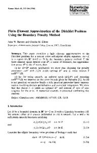
tational results are well matched with the analytical result (5.51). Example 2. We consider a four-to-one contraction domain, as depicted in Figure 1. Fluid flows from left to right, and this domain is characterized by the sudden width reduction of 75%. The boundary Γ is divided into four parts: the inflow boundary Γin , the wall boundary Γwall , the outflow boundary Γout , and the symmetry boundary Γsym (so that Γ = Γin ∪ Γwall ∪ Γout ∪ Γsym ). Let n and t be the unit outward normal and tangential vectors to Γ, respectively. Let π be the total stress. Then the boundary conditions are as follows [10]. • Inflow boundary Γin : u =

uin ,

T

Tin .

=

• Wall boundary Γwall : u = 0, ∇T · n = 0.

438


5

Γwall 4

y

3

2

Γin

Γwall

Ω

Γwall 1

Γout 0

−1

Γsym 0

5

10

15

20

x

Figure 1. Example 2: Computational domain Ω. • Outflow boundary Γout : u = ∇T · n =

uout , 0.

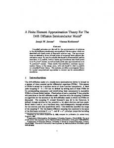
• Symmetry boundary Γsym : u · n = 0, ∇T · n = 0, π : nt = 0. Notice that we can interpret ∇T · n = 0 as an insulated boundary condition, u = 0 as the fluid does not move if it touches the wall, and that the condition u · n = 0 along Γsym implies that the flow in this half of the domain does not affect the flow in the other ‘half’ of the domain. The condition π : nt = 0 along Γsym is interpreted as a vanishing tangential contact force. We then set " ³ ¡ ¢2 ´ # · ¸ 24(1 − y 2 ) 6 1 − y4 uin = , uout = 0 0 5 Tin = 540 + y. 2 R Note that Γ u · n dΓ = 0 for the incompressibility condition ∇ · u = 0. The equations are simulated, and typical profiles for velocity, temperature, and pressure are presented in Figures 2 and 3. 7. Concluding remarks In this paper, the finite element solution of the non-isothermal Stokes-Oldroyd problem was investigated. We proved that a bounded approximate solution exists and also derived an error estimate for the solution. As mentioned earlier, this work is our initial step toward the numerical study of the equations governing non-isothermal viscoelastic flows characterized by, for example, the Oldroyd-B or Giesekus constitutive model. There are numerous engineering publications (for example, [9, 10, 11]) which consider non-isothermal viscoelastic flows and related application problems. However, further mathematical and numerical analysis of the problem is needed due to the complexity of the model equations. Details concerning numerical analysis and other computational issues will be addressed in a later paper.

FEM FOR NON-ISOTHERMAL STOKES-OLDROYD FLOW Contour plot of u

439

Contour plot of u

1

2

4

4

−0.5

20 3.5

3.5

−1

18 3

16

−2

14

2.5

−1.5

3

2.5 −2.5

2

y

y

12 2

10 1.5

−3 1.5

8

−3.5

6 1

1

−4

4 0.5

−4.5

0.5 2

−5 0

0

2

4

6

8

10 x

12

14

16

18

0

20

0

0

2

4

6

8

(a) u1 (x, y)

10 x

12

14

16

18

20

(b) u2 (x, y)

Figure 2. Solution profiles of the components of velocity.

Contour plot of T 4

549

3.5

548

547

3

546 2.5

y

545 2 544 1.5 543 1 542 0.5

0

541

0

2

4

6

8

10 x

12

14

16

18

20

540

Figure 3. Solution profile of temperature.

References [1] R. Armstrong, R. Bird, O. Hassager, Dynamics of Polymeric Liquids, Volume One, John Wiley and Sons, New York, 1987. [2] J. Baranger, D. Sandri, A Formulation of Stoke’s Problem and the Linear Elasticity Equations Suggested by the Oldroyd Model for Viscoelastic Flow, Mathematical Modelling and Numerical Analysis, 26, pp.331-345, 1992. [3] J. Boland, W. Layton, Error Analysis for Finite Element Methods for Steady Natural Convection Problems, Numerical Functional Analysis and Optimization, 11, pp.449-483, 1990. [4] S. Brenner, L. Scott, The Mathematical Theory of Finite Element Methods, Springer-Verlag, New York, 1996. [5] A.E. Caola, Y. Joo, R.C. Armstrong, R.A. Brown, Highly parallel time integration of viscoelastic flows, Journal of Non-Newtonian Fluid Mechanics, 100, pp.191-216, 2001. [6] V. Girault, P. Raviart, Finite Element Approximation of the Navier-Stokes Equations, Springer-Verlag, New York, 1979. [7] M. Gunzburger, L. Hou, T. Svobodny, Heating and Cooling Control of Temperature Distributions Along Boundaries of Flow Domains, Journal of Mathematical Systems, Estimation and Control, 3 No.2, pp.147-172, 1993. [8] M. Joshi, B. Bose, Some Topics in Nonlinear Functional Analysis, John Wiley and Sons, New York, 1985. [9] K. Kunisch, X. Marduel, Optimal Control of Non-Isothermal Viscoelastic Fluid Flow, Journal of Non-Newtonian Fluid Mechanics, 88, pp.261-301, 2000.

440


[10] Y. Joo, J. Sun, M. Smith, R. Armstrong, R. Brown, R. Ross, Two-Dimensional Numerical Analysis of Non-Isothermal Melt Spinning With and Without Phase Transition, Journal of Non-Newtonian Fluid Mechanics, 102, pp.37-70, 2002. [11] G.W.M. Peters, F.T.O. Baaijens, Modelling of non-isothermal viscoelastic flow, Journal of Non-Newtonian Fluid Mechanics, 68, pp.205-224, 1997. Department of Mathematical Sciences, Clemson University, Clemson, SC 29634, USA E-mail: [email protected] URL: http://www.math.clemson.edu/facstaff/clcox.htm Department of Mathematics, Clemson University, Clemson, SC 29634, USA E-mail: [email protected] URL: http://www.math.clemson.edu/facstaff/hklee.htm Department of Mathematics, Clemson University, Clemson, SC 29634, USA E-mail: [email protected]