finite element-based algorithms to make cuts for ... - PIER Journals

Progress In Electromagnetics Research, PIER 32, 207–245, 2001

FINITE ELEMENT-BASED ALGORITHMS TO MAKE CUTS FOR MAGNETIC SCALAR POTENTIALS: TOPOLOGICAL CONSTRAINTS AND COMPUTATIONAL COMPLEXITY P. W. Gross Mathematical Sciences Research Institute 1000 Centennial Drive, Berkeley, CA 94720, USA P. R. Kotiuga Department of Electrical and Computer Engineering Boston University 8 Saint Mary’s St., Boston, MA 02215, USA Abstract—This paper outlines a generic algorithm to generate cuts for magnetic scalar potentials in 3-dimensional multiply-connected finite element meshes. The algorithm is based on the algebraic structures of (co)homology theory with differential forms and developed in the context of the finite element method and finite element data structures. The paper also studies the computational complexity of the algorithm and examines how the topology of the region can create an obstruction to finding cuts in O(m20 ) time and O(m0 ) storage, where m0 is the number of vertices in the finite element mesh. We argue that in a problem where there is no a priori data about the topology, 4/3 the algorithm complexity is O(m20 ) in time and O(m0 ) in storage. We indicate how this complexity can be achieved in implementation and optimized in the context of adaptive mesh refinement.

1 Introduction and Outline 1.1 Electromagnetic and Numerical Scenario 1.2 Are Cuts Worth the Trouble? 1.3 Outline

208

Gross and Kotiuga

2 Definitions and Development of Topological Tools 2.1 (Co)Homology Groups 2.2 Poincar`e-Lefschetz Duality via Explicit Constructions 2.3 The Isomorphism H 1 (R; Z)  [R, S 1 ] 3 The Variational Formulation of the Cuts Problem 4 The Connection between Finite Elements and Cuts 4.1 The Role of Finite Elements in a Cuts Algorithm 5 Computation of 1-Cocycle Basis 5.1 Definitions 5.2 Formulation of a 1-Cocycle Generator Set 5.3 Structure of Matrix Equation for Computing the 1Cocycle Generators 5.3.1 Fixing Im (∂1T ) 5.3.2 dim(N (U )) = β1 (R) 5.3.3 Sparsity of ∂2T and U 5.3.4 Block Partition and Sparsity of the Matrix Equation 5.4 The Size of U22 6 Summary and Conclusions Acknowledgment Appendix A. Mesh-Counting Arithmetic A.1 The Euler Characteristic χ(R) A.2 The Details behind Table 1.2 Appendix B. Why Finite Element Analysis of Magnetic Fields Is Easy Once Cuts Are in Hand References 1. INTRODUCTION AND OUTLINE In this paper we consider a generic finite element-based algorithm to make cuts for magnetic scalar potentials and investigate how the topological complexity of the three-dimensional region, which constitutes the domain of computation, affects the computational complexity of the algorithm. The algorithm is based on standard finite element theory with a novel computation required to deal with

Finite element-based algorithms to make cuts

209

topological constraints brought on by a scalar potential in a multiplyconnected region. Thus, implementation can be designed to exploit pre-existing finite element software. Regardless of the topology of the region, an algorithm can be implemented with O(m30 ) time complexity and O(m20 ) storage where m0 denotes the number of vertices in the finite element discretization. However, in practice this is not useful since for large meshes since the cost of finding cuts would become the dominant factor in the magnetic field computation. In order to make cuts worthwhile for problems such as nonlinear or time-varying magnetostatics, or in cases of complicated topology (e.g., braided, knotted, or linked conductor configurations, or even simple coils), an implementation of O(m20 ) time complexity and O(m0 ) storage is regarded as “ideal”. The obstruction to ideal complexity is tied up in the structure of the fundamental group of the region. One implementation was designed to have ideal complexity [29], however, the implementation has heuristic assumptions which make it generally inadequate for making cuts in regions for which the fundamental group of R has a nontrivial commutator subgroup [13, 15]. This paper details an algorithm that can be implemented with O(m20 ) time complexity and 4/3 O(m0 ) storage complexity given no more topological data than that contained in the finite element connection matrix. While cuts algorithms have been discussed by several authors [7, 18, 37, 20, 21] some algorithms are based on the assumption that cuts can be made in analogy to branch cuts in complex analysis. Such algorithms are limited to problems reducible to a planar problem and their success for this limited class of problems hinges on the fact that the topology of 2-d surfaces is “perfectly understood.” In three dimensions, intuition from Amp`ere’s law leads to a formal definition of cuts in terms of a basis of the (abelian) homology groups of the region [20, 21, 15], even though such cuts do not necessarily render the region simply-connected [15]. The abelian nature of homology groups makes the problem computationally tractable while avoiding the subtle aspects of 3-dimensional topology which are trivial in two dimensions. 1.1. Electromagnetic and Numerical Scenario The proper context for the algorithm of this paper is in variational principles, the finite element method, and their connection to the topology of the domain of computation. Before seeing how topology enters the picture when going after a scalar potential, we define “magnetoquasistatics” as the class of electromagnetics problems where the magnetic field is described by a limiting case of Maxwell’s

210

Gross and Kotiuga

equations:  B · dS = 0

(1)

∂V



 H · dl = ∂S



J·n  ds

(2)

S

d E · dl = − dt ∂S


 S


B·n  ds

(3)

Here ∂V refers to the boundary of a region V and ∂S is the boundary of a surface S. The displacement current ∂D/∂t in Amp`ere’s law is neglected and the current density vector J is assumed to be solenoidal. The magnetic flux density vector B is related to the magnetic field intensity H by B = B(H), or for linear isotropic media, B = µH. The current density J in conductors is related to the electric field intensity vector E by Ohm’s law: J = σE. Let R denote a region which is the intersection of the region where it is desired to compute the magnetic field and where the current density J is zero. In R, curl H = 0,

(4)

so that in terms of a scalar potential ψ, H = grad ψ

(5)

in any contractible subset of R but ψ is globally multivalued as seen via Amp`ere’s Law and illustrated in Figure 1. Some scalar potential formulations sidestep the issue of the multivalued scalar potential by expressing the magnetic field as H =  where Hp is a particular solution for the field obtained, Hp + grad ψ, say, from the Biot-Savart Law. However, in this case, if B = µH and  leading to significant µ → ∞, then H → 0 so that Hp = −grad ψ, cancellation error for computation in regions where H  0 while a “total” scalar potential as in (5) eliminates cancellation error. In addition, integration of the Biot-Savart integral destroys the sparsity of any discretization. The particular solution, Hp , can be set to zero in a multiply-connected region when one introduces the notion of a “cut” which makes the scalar potential single-valued and if the software to generate cuts does not require input from the user. This is a major incentive for developing such algorithms.

Finite element-based algorithms to make cuts

211

c2 S c I

c1

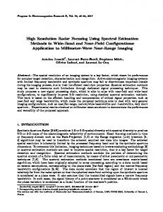
Figure 1. A current-carrying trefoil knot c with current I and cut S. If H = grad ψ, Amp`ere’s Law implies  that a scalar potential ψ is multivalued as illustrated with loop c1 : c1 H · dl = I ⇒ ψ multivalued  when there is no cut. On the other hand, c2 H · dl = I − I = 0, even though c2 is not contractible to a point so that c2 gives no information about ψ. With the cut in place (as shown) imposing a discontinuity I in ψ from one side of the cut to the other makes ψ singlevalued on the cut complement. Note that Amp`ere’s law does not require that c2 intersect the cut. 1.2. Are Cuts Worth the Trouble? In order to evaluate the utility of having cuts, one must also compare computational overhead with the expected acceleration in solution time. Given a finite element mesh it is possible to compare the solution time complexities of the associated finite element matrix equations for scalar potential and vector methods. Since semidirect matrix solvers are commonly used for large problems, we argue in terms of a conjugate gradient (CG) solver iteration for the finite element matrix equations (c.f. Appendix A). Let F0s denote the number of floating point operations (FLOPs) per conjugate gradient solver iteration for nodal interpolation of a scalar potential on a tetrahedral mesh. Similarly, let F0 and F1 respectively denote the number of FLOPs per CG iteration for node- and edge-based vector interpolation [25]. Finally, let X0s , X0 , and X1 denote the number of nonzero entries in the stiffness matrix for nodal interpolation of a scalar potential, and node- and edge-based vector interpolation, respectively. Assuming similar distributions of eigenvalues in the matrices, the convergence of CG for each matrix is the same and the ratio of the complexity of the CG iterations is a reflection of the ratio of computer run times. Table 1.2 summarizes how vector formulations compare to a scalar potential formulation. This has been confirmed experimentally by Saitoh [33]. The “mesh-counting arithmetic” used to derive Table 1 is

212

Gross and Kotiuga

X/X0s F/F0s

Node (X0 & F0 ) 9 7.5–7.6

Edge (X1 & F1 ) 7.5 9.7–10.7

Table 1. Relative number of nonzero entries in the stiffness matrix (X) and number of floating point operations (F ) per CG iteration for node- and edge-based vector interpolation compared to scalar potential (X0s and F0s ) on large tetrahedral meshes. summarized in Appendix A. If a scalar potential can be computed, it provides a substantial speed-up, but the overhead is that of computing cuts. Hence, cuts may be most useful in the context of time-varying or nonlinear problems where cuts are computed only once but iterative solutions are required for the field. Algorithm design must begin with the choice of an algebraic framework for the computation, and for reasons of computability, this is the most critical choice. The often-made assumption that cuts must render the region simply-connected forces one to work with a structure called the first homotopy group for which basic questions related to this group are not known to be algorithmically “decidable”. In practical terms, homotopy-based algorithms are limited to problems reducible to a planar problem. Thus, their success depends on the fact that 2-d surfaces are completely classified (up to homeomorphism) by their Euler characteristic and numbers of connected components and boundary components. The (co)homology arguments presented here lead to a general definition of cuts and an algorithm for computing them by linear algebra techniques, but when using sparsity of the matrices to make the computation efficient, homotopy emerges as an important and useful tool. 1.3. Outline With the preceding motivation in mind, we outline the main sections of this paper. Section 2 introduces the essential pieces of (co)homology theory and differential forms required for defining the notion of cuts and for finding an algorithm to compute them. Section 3 presents a variational formulation which can be used in the context of the finite element method. Section 4 describes the algorithm in the context of finite elements, and gives the finite element equations, but one essential computation, that which depends on the topological structure of the region, is left for Section 5. Section 5 fills in the piece missing

Finite element-based algorithms to make cuts

213

from Section 4, describing an algorithm for finding the topological constraints on the variational problem, and gives an analysis of the computational complexity of finding cuts. The overall process of computing cuts is summarized in algorithm 1 and the algorithm of Section 5 is summarized in algorithm 2. Two example problems are considered in order to illustrate the obstruction to O(n) complexity. Section 6 concludes with a summary of the main results, a review of geometric insights used to reduce the complexity of the algorithm, and suggestions for future work. 2. DEFINITIONS AND DEVELOPMENT OF TOPOLOGICAL TOOLS The subtleties of 3-dimensional electromagnetic boundary value problems are articulated through some special algebraic structures and relationships between them. A good technical exposition of these is available from many sources [19, 10, 12, 35, 32], and there is a historical context for their use in electromagnetic theory [27, 4], yet they seem to be virtually absent from finite element algorithm design. We consider the essential points here, reviewing three ingredients required for an algorithm: (i) Homology and Cohomology groups: Homology groups are the structures which algebraically encode information describing current-linking (as in Amp`ere’s law) as well as cuts while cohomology groups describe curl-free vector fields in the region of interest. (ii) Poincare-Lefschetz duality makes a connection between the curlfree fields and homology classes describing cuts, hence a definition of cuts. (iii) Isomorphism H 1 (R; Z)  [R, S 1 ]: A relationship between the curlfree fields and maps from the nonconducting region to the circle which guarantees existence of cuts with some desirable properties and is the key to a variational formulation of a cuts algorithm. There are several advantages to formulating cuts in terms of (co)homology groups. One is that when a constructive proof of the existence of cuts is phrased in terms of the formalism of a certain homology theory, the proof gives way to a variational formulation for a cuts algorithm [21]. Another advantage is that various homology theories give several ways to view cuts. Regarding a finite element mesh as a simplicial complex [10], simplicial homology theory provides a framework for implementing an algorithm to make cuts and even determines the most natural data structures as described in a

214

Gross and Kotiuga

companion paper [14] whose results are used in Section 5. Except for portions based on standard finite element theory, an implementation of the algorithm uses only integer arithmetic, thus avoiding introduction of rounding errors associated with real arithmetic [29, 13]. 2.1. (Co)Homology Groups We take R to be the nonconducting region with boundary ∂R; the complement of R relative to R3 , denoted by Rc , is the union of the problem “exterior” and the conducting region. Noting that Amp`ere’s law is a statement about closed loops in R which link nonzero current [15], we define the first homology group of R with integer coefficients, denoted by H1 (R; Z), as the group of equivalence classes of closed loops in R which link closed paths in Rc which may be current paths [15]. Two closed loops in R lie in the same equivalence class if together they comprise the boundary of a surface in R (Figure 2).

S R

R

S
c1

c2

c
I

I

(a)

(b)

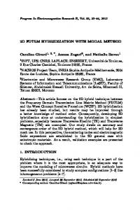
Figure 2. In (a), closed loop c1 lies in R but is not the boundary of a surface in R. However, c1 and c2 together comprise the boundary of a tube S, thus c1 ∼ c2 ; c1 and c2 are nonbounding 1-cycles. In (b), loop c
links zero net current and is the boundary of surface S
(disk with handle), thus while ∂c
= 0, c
= ∂S
, so c
is a bounding 1-cycle but it is not contractible to a point in the complement of the knot.

Finite element-based algorithms to make cuts

215

More generally, the first homology group is conceived by taking linear combinations of closed loops in R modulo curves which are boundaries of surfaces in R. In this context, 1-boundary refers to a closed loop which is the boundary of a surface in R, c = ∂2 S, where ∂2 is the boundary operator on surfaces. The term 1-cycle refers to a closed loop with zero boundary ∂1 c = 0. Boundaries are cycles, but not all cycles are boundaries, thus H1 (R) comes about as a quotient space of cycles modulo boundaries. In other words, given any S, ∂1 (∂2 S) = 0, the boundary of a boundary is zero, however it is not necessarily true that every closed curve is the boundary of some surface lying in R. Hence it is the “equivalence classes of nonbounding cycles” which are nontrivial in the quotient space. The Z in H1 (R; Z) expresses the fact that in this case there is no loss of information if one builds H1 by taking only integer linear combinations of closed loops [15]. (As shown in [20], the homology groups for R are torsion-free so that integer coefficients are sufficient.) The number of independent closed nonbounding loops (number of generators or “rank” of H1 ) is called the first Betti number of R (Maxwell [27] and Kirchoff’s “cyclomatic number”) and is denoted by β1 (R). β1 (R) is a characteristic parameter of R and is significant because it describes the number of independent closed loops in R which link nonzero current, and as such will characterize the number of variational problems to be solved in the cuts algorithm. Dual to H1 (R) is the first cohomology group of R, denoted by H 1 (R; Z). This can be regarded as the group of curl-free vector fields in R modulo vector fields which are the gradient of some function. As in the case of H1 , it is enough to take “forms with integer periods” meaning that integrating the field about a generator of H1 gives an integer. The rank of H 1 (R; Z) is also β1 (R). In three dimensions, H1 (R) and H 1 (R) formalize Amp`ere’s law in the sense that, respectively, they are algebraic structures describing linking of current and irrotational fields in R due to currents in Rc . The second relative homology group of R modulo the boundary of R, denoted by H2 (R, ∂R; Z), is the group of equivalence classes of surfaces in R with boundary in ∂R. Classes in H2 (R, ∂R; Z) are surfaces with boundary in ∂R but which are not themselves boundaries of a volume in R. Its rank is the second Betti number, β2 (R, ∂R) (Maxwell’s “periphractic number”). H2 (R, ∂R; Z) is the quotient space of surfaces which are 2-cycles up to boundary in ∂R modulo surfaces which are boundaries (Figure 3). In 3-d these turn out to be surfaces used for flux linkage calculations, and in fact turn out to be a family of cuts. This will be shown precisely but we need to start with the definition to get to the algorithm. However, the fact that these are cuts

216

Gross and Kotiuga

R

S ∂S I

Figure 3. S is a surface in R with ∂S ∈ ∂R, but S is not the boundary of a volume in R. Also see Figure 1. can be understood intuitively by noting that an essential requirement for a set of cuts is that they must break every loop which links current in the sense of Amp`ere’s law. For this to occur, the boundaries of the cuts must be on the boundary of the region, in this case ∂R. Thus we expect to have at least β1 (R) cuts. This is a geometric and intuitive way of understanding what cuts are, but it does not establish their existence or give a way of computing them. The tools described in the following sections give the required formalism for both. 2.2. Poincar` e-Lefschetz Duality via Explicit Constructions The second ingredient in the formulation of cuts is a “duality theorem” which relates H 1 (R; Z) to H2 (R, ∂R; Z) in three dimensions and will lead to a variational formulation of cuts. At first, we define spaces so that a special case of Poincar`e-Lefschetz duality can be written in terms of vector fields. Later it will be stated generally in terms of differential forms to show that this construction is general. Let    (6) F = F | curl F = 0 in R, F · dl ∈ Z c

for a closed path c where ∂c = 0 (nonbounding 1-cycle), and G = {G | div G = 0 in R, G · n =0 on ∂R}.

(7)

Given any surface S used to calculate flux linkage, Poincar`e-Lefschetz duality says that there exists an FS ∈ F dual to S such that   FS · G dV = G·n  dS (8) R

S

Finite element-based algorithms to make cuts

217

for all G ∈ G. This illustrates the fact that the space of H 1 (R; Z) and H2 (R, ∂R; Z) are dual spaces of the space of G vector fields subject to the following equivalence relation: G ∼ G
if G
= G + curl A

(9)

for some A where n  × A = 0 on ∂R. In the preceding, H 1 (R) has been articulated in terms of vector fields for an intuitive understanding of the structure. However, the theory is developed rigorously in terms of differential forms, so these are introduced here in order to exploit the general theory. Loosely speaking, differential forms are the objects appearing under integral signs – integrands of p-fold integrals in an n-dimensional manifold where 0 ≤ p ≤ n. They generalize the notion of a vector field and are a natural framework for engineering electromagnetics [19, 11]. For an n-dimensional manifold M n , the set of all p-dimensional regions c over which p-fold integrals are evaluated is denoted by Cp (M n ) while the set of all p-forms ω are denoted by C p (M n ). Since Cp (M n ) and C p (M n ) are spaces with some algebraic structure, integration  ω (10) c

can be regarded as a bilinear map  : Cp (M n ) × C p (M n ) −→ R

(11)

(which, in a definite sense, is a nondegenerate bilinear pairing between the spaces). In this context, the fundamental theorem of calculus, Gauss’ and Stokes’ theorems of multivariable calculus, and Green’s theorem in the plane are generalized by the Stokes theorem on manifolds:   dω = ω (12) c

∂c

where ∂c ∈ Cp−1 (M n ) is the boundary of c and the exterior derivative operator d takes p-forms to p+1-forms so as to satisfy Stokes’ theorem. Finally, there is a bilinear, associative, graded commutative product of forms, called the exterior product, which takes a p-form ω and a q-form η and gives a p + q-form ω ∧ η. The introduction to homology groups hinted at the fact that ∂p−1 ∂p c = 0. By a simple calculation, this combines with Stokes’ theorem to show that p-forms satisfy dp+1 dp ω = 0 and motivates

218

Gross and Kotiuga

the following definition. A form µ is said to be closed if dµ = 0. In vector calculus, this amounts to saying that curl grad φ = 0 and div curl A = 0. Moreover, the existence of nonbounding cycles and Stokes’ theorem also leads to the notion of exact forms: if µ = dω for some ω, µ is said to be exact. While all exact p-forms are closed, not all closed forms are exact, so H p is the quotient group of closed p-forms modulo exact p-forms. Formally, the coboundary operator is a map dp : C p (M ) → C p+1 (M ) and H p (M ; R) = ker dp /Im dp−1 .

(13)

In general, Poincar´e-Lefschetz duality says that for a compact, orientable n-dimensional manifold with boundary, M n , H k (M n ; Z)  Hn−k (M n , ∂M n ; Z)

(14)

for 0 ≤ k ≤ n. This theorem is true for any abelian coefficient group, but it is enough to deal with integer coefficients here. In the case of n = 3, duality establishes a one-to-one correspondence between classes in H 1 (R; Z) and classes in H2 (R, ∂R; Z). In the context of magnetoquasistatics, these are, respectively, equivalence classes of magnetic fields and equivalence classes of surfaces for flux linkage calculations. To develop a formal definition of a “cut” we need the notion of the Poincar´e-Lefschetz dual of a submanifold. Given an n-dimensional compact, oriented manifold M n with boundary, a closed oriented n−kdimensional submanifold S of M n , and a closed n − k-form ω whose restriction to ∂M is zero, the Poincar´e-Lefschetz dual of S is a closed k-form ηS such that [6]   ω ∧ ηS = ω. (15) Mn

S

This is a generalized statement of equation (8). When subjected to the (co)homology equivalence relations, the bilinear pairings on both sides of equation (15) become nondegenerate bilinear pairings between H k (M n ) and H n−k (M n , ∂M n ) on the left, and Hn−k (M n , ∂M n ) and H n−k (M, ∂M ) on the right. Thus equation (14) arises since H n−k (M n , ∂M n ) is the dual space to both spaces. In other words, for the homology class [S] ∈ Hn−k (M n , ∂M n ) associated with a submanifold S ∈ M n , there is an associated unique cohomology class [ηS ] ∈ H k (M n ). As a consequence of Poincar´e-Lefschetz duality, cuts can be defined as representatives of classes in H2 (R, ∂R; Z). The isomorphism discussed below allows us to restrict our attention to cuts which are embedded manifolds in R, and at the same time gives a way of computing these cuts through a variational problem.

Finite element-based algorithms to make cuts

219

2.3. The Isomorphism H 1 (R; Z)  [R, S 1 ] The third ingredient required for an algorithm is the relationship between H 1 (R; Z) and maps from R to the circle, S 1 , where we think of S 1 as the unit circle in the complex plane. Let [R, S 1 ] denote the space of maps f : R → S 1 up to the equivalence relation given by homotopy. Then, H 1 (R; Z)  [R, S 1 ]

(16)

which says that the group of cohomology classes of R with integer periods is isomorphic to the group of homotopy classes of maps from R to S 1 [20]. The reason for introducing (16) is twofold: First, we have no guarantee that homology classes can be represented by manifolds (surfaces). As discussed below, equation (16) gives this guarantee. Second, since it associates each class in H 1 to a class of maps from R to S 1 , a suitable choice of energy functional on [R, S 1 ] will give a variational problem and an algorithm for computing cuts. Hence, this isomorphism and Poincar´e-Lefschetz duality give way to an algorithm for cuts. Concretely, choosing µ = dθ/2π, a closed, nonexact 1-form on S 1 , then f ∗ (µ) is the “pullback” of µ via f so that one can regard f ∗ (µ) as monitoring the change in θ as one covers a family of cuts in R. Poincar´e-Lefschetz duality and the preimage theorem [16] say that for a regular point p of f on S 1 ,   dθ ω ∧ f ∗( ) = ω (17) 2π R f −1 (p) for any closed 2-form ω. Thus, given f : R → S 1 where f winds around S 1 , the pullback f ∗ (µ) is the Poincar´e-Lefschetz dual to f −1 (p) [20]. In terms of vector calculus, given a map f : R → S 1 , equation (17) can be re-written as   1 G · grad (ln f )dV = G·n  dS (18) 2πi R f −1 (p) for any G ∈ G. When G = µH and H = 1/2πi grad (ln f ), each side of equation (18) can be regarded as an expression for the energy of a system of (unit) currents in R3 − R. In particular, note that the right hand side is the integral over a cut of the magnetic flux due to a unit current.

220

Gross and Kotiuga

3. THE VARIATIONAL FORMULATION OF THE CUTS PROBLEM On the basis of the tools introduced above, the computation of cuts can be formulated as a novel use of finite elements subject to two constraints imposed by the topology of R. The idea is to come up with a variational problem for finding minimum energy maps f from classes in [R, S 1 ]. Hence, a principle for finding cuts is to compute a collection of maps, fq : R → S 1 , 1 ≤ q ≤ β1 (R) which correspond to a basis of the first cohomology group with integer coefficients H 1 (R; Z) and by duality, to a basis for H2 (R, ∂R; Z). Any map in the homotopy class can be used, but picking harmonic maps reduces the problem to quadratic functionals tractable by the finite element method. Furthermore, the level surfaces of these maps are nicer than in the generic case. As a variational problem, finding cuts can be rephrased as follows [21]. “Computing maps” means finding the minima to β1 (R) “energy” functionals  grad fq∗ · grad fq dR, 1 ≤ q ≤ β1 (R) (19) F (fq ) = R

subject to two constraints: fq∗ fq = 1 in R and, for the jth cut, 1 ≤ j ≤ β1 (R),  1 grad (ln fj ) · dl = Pjk 2πi zk

(20)

(21)

where {zq }, 1 ≤ q ≤ β1 (R), defines a set of generators of H1 (R) and Pjk is the period of the jth 1-form on zk is an entry of a nonsingular period matrix P . Intuitively, one might require the period matrix to be the identity matrix, but this is overly restrictive for a practical implementation of the algorithm. In fact, as discussed in Section 5, direct computation of a basis for H1 (R) is impractical but an equivalent criterion can be used to satisfy the constraint imposed by H1 (R). The solution to each map in the variational problem is unique since the “angle” of each fq is a (multivalued) harmonic function which is uniquely specified by equation (21) [15]. When the functionals are minimized, a set of cuts is computed by the formula Sq = fq−1 (pq )

(22)

Finite element-based algorithms to make cuts

221

where pq is any regular value of fq , 1 ≤ q ≤ β1 (R). Note that Sq is the Poincar´e-Lefschetz dual to d(ln f /2πi), as seen in equation 17 [20]. On any contractible subset of R, constraint (20) is satisfied by letting fq = exp(2πiϕ), 1 ≤ q ≤ β1

(23)

where ϕ is some real, locally singlevalued, but globally multivalued, differentiable function. Choosing fq this way, the Euler-Lagrange equation of (19) is Laplace’s equation [15]. Equation (23) is satisfied on open, contractible subsets Ui and their intersections. When the Ui form a cover of R, the global problem is assembled by considering the combinatorics of intersections Ui as noted in [6, §13] and also described in [17] in the context of the Cousin problem in complex analysis. For a computer implementation using standard data structures, it is sufficient to take a (tetrahedral) discretization of R and consider what happens across faces of the tetrahedral elements. Using the normalized angle of fq [21], θq = (ln fq /2πi)

mod 1

(24)

on an element and interpolating θq linearly over each element, we must consider that (21) prevents θq from being globally well-defined. Section 5 addresses how constraints (21) are handled without making explicit reference to a set of curves representing a basis for H1 (R). However, we begin by considering constraint (20) and the finite element-based part of the algorithm in the next section. Since each of the β1 problems is treated in the same way, in the next section we drop the subscript denoting the qth variational problem in order to simplify notation. 4. THE CONNECTION BETWEEN FINITE ELEMENTS AND CUTS Here we consider the variational problems for (any) one of the β1 (R) maps fi representing a class in H2 (R, ∂R) (by duality) and how the variational problem is handled via the finite element method. While the principles behind computing cuts are not dependent on the type of discretization used, this section is set in the context of first-order nodal variables on a tetrahedral finite element mesh as the data structures are simple. 4.1. The Role of Finite Elements in a Cuts Algorithm Consider a tetrahedral discretization of R, denoted by K, with m3 elements, m0 nodes. The ith tetrahedron in K is denoted by σi3 .

222

Gross and Kotiuga

Recalling equations (23) and (24), let θ be discretized on each element by the set θji , 1 ≤ i ≤ m3 , 1 ≤ j ≤ 4 for each one of the β1 (R) variational problems. Here the subscript refers to the jth node of the ith tetrahedron and the θji on individual elements are defined modulo integers since we seek a map into the circle. Furthermore, constraints (21) require that there be discontinuities in θji between pairs of adjacent elements. This is not a problem since the finite element connection process is modified accordingly as described below. To make a bridge to the finite element method, we also let uk , 1 ≤ k ≤ m0 denote a potential discretized on nodes of the mesh [21]. a

a

ζ lij σi3

σj3 c

c b

b

l

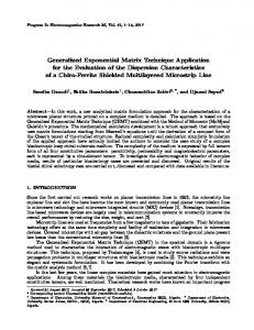
Figure 4. Jump ζkij is imposed across face shared by elements i and j and Jai − Jaj = ζ lij . The usual finite element connection matrix is defined as  1 if global node k is the jth local node in σi3 i Cjk = 0 otherwise

(25)

The modified connection process is the marriage, via the finite element connection matrix, of variables defined locally on the nodes of individual elements (θji ) to variables defined on the global node set of the mesh (uk ). Consequently, variables defined element-by-element are said to be on the unassembled mesh while those defined on the global nodes are on the assembled mesh. Global constraints (21) are handled via nodal discontinuities on the unassembled mesh, Jji , 1 ≤ i ≤ m3 , 1 ≤ j ≤ 4 (Figure 4). The jumps are specified so that for a given global node, Jji is an integervalued jump relative to a Jlk which is set to zero. From the perspective of a global node, there is a set of Jji associated with the global node (one Jji per element in which the global node is a local node), and

Finite element-based algorithms to make cuts

223

one Jji per set can be set to zero. Then θji , which is defined on the unassembled mesh, is written θji =

m0

i Cjk uk + Jji

(26)

k=1

1 ≤ i ≤ m3 , 1 ≤ j ≤ 4. Note that for each of the β1 (R) variational problems, there is one set of variables Jji . To finish specifying θji , the relationship between sets Jji and the homology class of the corresponding cut is needed. Recall that the sets of local nodal jumps Jji are defined on the unassembled finite elements problem. Since the discontinuity in θ must be consistent across the face of a tetrahedron, we introduce a set of discontinuities across faces, ζ l , 1 ≤ l ≤ m2 where m2 is the number of faces in the mesh. These are illustrated in Figure 4. Since there are β1 variational problems there is a set {ζ1l , . . ., ζβl 1 }, and for the kth cut, given ζki , the remaining Jji can be found by the back substitution l

i − Jnj = ζkij Jm

(27)

when elements i and j share face lij . The “topological computation” relating face jumps ζk to the relative homology class of the kth cut is discussed in Section 5. At this point, if one is interested in using a scalar potential, but not in making the cuts visible to the user as a diagnostic tool, the set of face jumps {ζ1 , . . ., ζβ1 } is a set of cuts. However, note that these cuts are not embedded manifolds, but nonetheless represent a basis for H2 (R, ∂R; Z). We will see in Section 5 that the face jumps can be identified with a class in the simplicial homology group related to H2 (R, ∂R). On the basis of the variational problem defined in equations (19)–(21), “finite element analysis” can be used to solve for each of β1 (R) potentials, uk . On each connected component of R, begin by setting one (arbitrary) variable in uk to zero. Then define barycentric coordinates λli , 1 ≤ i ≤ 4, on the lth tetrahedron, σl3 , and build the l : element stiffness matrix Kmn  l Kmn = grad λlm · grad λln dV. (28) σl3

Discretizing the normalized angle θ (24) on σl3 by θl =

4

i=1

λli θil ,

(29)

224

Gross and Kotiuga

and substituting into the functional (19), gives F (θ) = 4π 2

m3

4 4



l l l θm θn Kmn .

(30)

l=1 m=1 n=1

Using equation (26) to “assemble the mesh” gives a quadratic form in uk . The minimum of the quadratic form is obtained by differentiating with respect to the uk , resulting in the following matrix equation: m0

Kij ui = −fj

(31)

i=1

Here {Kij } forms the usual stiffness matrix: m 4 4 3

l l l Kij = Cnj Kmn Cmi

(32)

l=1 m=1 n=1

and, by equation (27), the source term m 4 4 3

l l Jnl Kmn Cmj fj = ,

(33)

l=1 m=1 n=1

is related to the homology class of a relative cycle in H2 (R, ∂R) by means of {ζji }. Thus, with the exception of computing {ζji } and forming source term (33), the algorithm is readily implemented in any finite element analysis program. This gives the maps from R to S 1 . To find the cut, recall Poincar´e-Lefschetz duality and equation (22). For each connected component of R, i (uk + c) mod 1. (θ
)ij = Cjk

(34)

where c is a constant so that θ
= 0 is a regular value of f . After solving β1 (R) variational problems, we proceed element by element to find and plot fq−1 (θ
= 0), 1 ≤ q ≤ β1 (R) to obtain a set of cuts. This is done in an unambiguous way if the mesh is fine enough to ensure that, over an element, θji does not go more than one third of the way around the circle. In order to use the cut for a scalar potential computation (c.f. Appendix A.2), the cut must be specified in terms of internal faces of the mesh, much as sets ζi are defined. For this we define β1 sets Si of faces obtained by perturbing a level set of the harmonic map onto internal faces of the finite element mesh. On a tetrahedral mesh this

Finite element-based algorithms to make cuts

225

level set u = s Figure 5. Level set of harmonic map is perturbed in gradient direction onto a face of the tetrahedral element. The face is selected merely by virtue of the fact that the potentials u(vi ≥ s) where vi is the ith vertex. In other words, the direction of grad u defines a normal to the cut, but it is unnecessary to actually compute the gradient. Cases in which the level set is perturbed onto an edge or vertex of the tetrahedron can be ignored since the level set will perturb onto the face of a neighboring tetrahedron. is done by simply choosing the element face which is on the side of the level set indicated by the normal (gradient direction) when the level set passes through the element. This is illustrated in Figure 5. Besides computing the {ζ1 , . . ., ζβ1 } and incorporating the Sq as subcomplexes of the mesh, the computation of cuts makes use of standard software found in finite element software packages. Although the sign of a floating point calculation is required at one step, the “topological” part of the code is otherwise implemented with integer arithmetic and is therefore immune to rounding errors. The following “algorithm” shows how cuts software fits into the typical finite element analysis process. The second and third steps are not ”standard” FE software, but are implemented with integer arithmetic and thus avoid introducing rounding error. Algorithm 1 (Finite elements and cuts) (1) Tetrahedral mesh generation and refinement (2) Extraction of simplicial complex: Employ the data structures from [14] and generate the data needed for computing interelement constraints ζi . (3) Topological processing: Compute interelement constraints {ζ1 , . . ., ζβ1 } defined in equation (27) and described in Section 5 and algorithm 2. (4) Finite element solution: Use (32) and (33) to form (31) for each

226

Gross and Kotiuga

of β1 variational problems, and solve them by the finite element method. (5) Obtain cuts: Level sets of the harmonic maps computed in the last step are cuts. When perturbed onto the 2-skeleton of the mesh to define β1 surfaces Si , they are the data needed to do a magnetic scalar potential calculation. 5. COMPUTATION OF 1-COCYCLE BASIS Now we consider the computation of the interelement constraints which come about as a result of constraint (21) on the variational problem and were defined in equation (27). The computation must be in terms of the finite element discretization K, and as indicated at the beginning of Section 2, simplicial (co)homology is the algebraic framework. Here we use the results of companion paper [14] which describes the simplicial complex, and how it generates the finite element data structures required for computing cuts when taking the view that K and its simplicial complex are the same thing. In [14], we discuss the duality between the boundary homomorphism on a simplicial complex K and its dual complex DK and show that the duality appears naturally in the data structures describing K. This duality is a discrete version of Poincar´e-Lefschetz duality introduced in Section 2, but stated at the level of the simplicial chain complex (the algebraic structure which is most suited to describing finite element meshes). The dual complex is also the most appropriate structure for describing the computation of the topological constraints for the variational problem. Below we give the basic definitions needed to formulate the computation of the topological constraints. 5.1. Definitions For a tetrahedral mesh K, se denote the nodes, edges, faces, and tetrahedra as 0-, 1-, 2-, and 3-simplexes, respectively, though in general it is possible to have an n-dimensional simplicial mesh. The total number of p-simplexes in a mesh is denoted by mp . Each set of p-simplexes forms a linear space with (for the present purpose) coefficients in Z, Cp (K; Z), called the p-chain group. There is a boundary homomorphism ∂p : Cp (K; Z) → Cp−1 (K; Z) which takes psimplexes to p−1-simplexes such that the composition of two successive transformations is zero: ∂i ∂i+1 = 0, 1 ≤ i ≤ n.

(35)

Finite element-based algorithms to make cuts

227

In other words, Im (∂i+1 ) ⊆ ker(∂i ), and the sequences in (35) are summarized in the simplicial chain complex: ∂

∂p

∂p−1

∂

n 1 · · · −→ Cp−1 (K) −→ · · · −→ C1 (K) −→ C0 (K) −→ 0. 0−→Cn (K) −→ (36)

As in the continuum case, this allows us to define homology (and cohomology) groups. The adjoint operator of the boundary homomorphism is the T : C p (K; Z) → C p+1 (K; Z) where C p (K; Z) coboundary operator ∂p+1 is the simplicial cochain group of functionals on p-chains; formally, C p (K; Z) = hom(Cp (K), Z). The cochain cp ∈ C p satisfies the relation T < cp , ∂p+1 cp+1 >=< ∂p+1 cp , cp+1 >

(37)

for any cp+1 ∈ Cp+1 . This is a discrete version of Stokes’ theorem (c.f. T . ∂T ∂T = 0 equations (12) and (13)) and serves as a definition of ∂p+1 i i+1 so that there is a cochain complex: ∂T

∂pT

T ∂p−1

∂T

n 1 · · · ←− C p−1 (K) ←− · · · ←− C 1 (K) ←− C 0 (K) ←− 0. 0←−C n (K) ←− (38)

Simplicial homology groups are quotient groups Hp (K) = ker(∂p )/Im (∂p+1 ) and the pth Betti number βp = Rank (Hp ) (c.f. Section 2.1); the simplicial cohomology groups are defined by T )/Im (∂ T ). An element of H p (K) is the coset H p (K) = ker(∂p+1 p ζ + Bp

(39)

where B p (K) = Im (∂pT ) is the p-coboundary subgroup of C p (K), T ) is a p-cocycle. The ranks of the homology and and ζ ∈ ker(∂p+1 cohomology groups are related: Rank (Hp ) = Rank (H p ). By identifying non-boundary p-simplexes in K with n − p-cells (i.e. when n = 3, 3-simplexes become nodes, 2-simplexes become edges, etc.), a formal dual of K, called the dual complex DK can be formed directly from the connection matrix describing K. (The boundary is excluded since there are no 3-simplexes in ∂K.) The dual DK is not simplicial but cellular, and the number of p-cells of DK is denoted by m ˘ p . DK is a cellular complex in the sense of (36). Poincar´e duality amounts to saying that the coboundary operators of the simplicial complex are dual to the boundary homomorphisms of the cellular complex, denoted by ∂˘p in the sense that T ∂p+1 = ∂˘n−p

(40)

228

Gross and Kotiuga

[14]. Thus, for a 3-dimensional complex, ∂˘3 =∂ T

∂˘2 =∂ T

∂˘1 =∂ T

0−→C3 (DK) −→1 C2 (DK) −→2 C1 (DK) −→3 C0 (DK) −→ 0 (41) and ∂˘T

∂˘T

∂˘T

3 2 1 C 2 (DK) ←− C 1 (DK) ←− C 0 (DK) ←− 0. 0←−C 3 (DK) ←−

(42)

The (co)homology of DK is isomorphic to the (co)homology of K in complementary dimensions. In other words, Poincar´e duality on the (co)chain level gives us the Poincar´e duality of Section 2. 5.2. Formulation of a 1-Cocycle Generator Set The duality between boundary and coboundary operators as set forth above is useful for formulating the outstanding problem of computing {ζ1 , . . . , ζβ1 } introduced in equation (27). These variables were introduced in order to handle interelement topological contraints (21) of the variational problem, but equation (21) cannot be applied directly since a set of generators for H1 (R) is generally not known beforehand and is hard to compute. On the other hand, (21) simply gives the periods of 1-cocycles integrated on a homology basis, so that it is enough to know a basis for the nontrivial (i.e. non-coboundary) 1cocyles. Here, the ζi are described by β1 (R) 1-cocycles which are generators for classes in H 1 (DK; Z), and by duality represent sets of faces having nonzero jumps in backsubstitution equation (27). The advantage of formulating the problem in terms of H 1 (DK; Z) is that it immediately yields a matrix equation, and the 1-cocycles form β1 (R) source terms for the righthand side of equation (31). In general, equivalence classes in H 1 (DK; Z), the first cohomology group of the dual complex with integer coefficients, can be represented by integer-valued 1-forms which are functionals on 1-cells of the dual mesh. However, it is only possible (and necessary) to compute, for each equivalence class, a generating 1-cocycle defined by two properties described below: First, to obtain a basis for non-cobounding 1-cocycles a basis for the 1-coboundary subgroup B 1 (DK; Z) must be fixed by constructing the image of a 0-coboundary map ∂˘1T : C 0 → C 1 . This not only fixes how B 1 (DK; Z) is represented, but allows the computation of 1-cocycles which represent closed, nonexact 1-forms. Second, by definition, the 1-cocycle must also satisfy the condition that on the boundary of each 2-cell in DK, ∂˘2 (2-cell) = 61 e1 + 62 e2 +

Finite element-based algorithms to make cuts

229

2-cell

root

2-cell

root (a)

(b)

Figure 6. 1-cells on maximal spanning tree (solid) and 2-cells in DK. In (a), the 2-cell cocycle condition has three free variables (those not on the tree) while in (b), the condition can be satisfied (trivially) in terms of variables on the tree. . . . + 6n en , < ζj , ∂˘2 (2-cell) >=

n

6i ζji (ei ) = 0

(43)

i=1

where 6i = ±1 denotes the orientation of the ith 1-cell on the boundary of the 2-cell (Figure 6). The condition must be satisfied on any simply-connected subset of the mesh, but the data readily available from the finite element connection matrix relates to 2-cells. Since Poincar´e duality for complexes K and DK (40) says that ∂˘2 and ∂2T are identified, the coboundary operator ∂2T is the incidence matrix of 2and 1-cells in DK and contains the data for the 1-cocycle conditions over all of DK. Equations (37) and (43) together say that for any 1-cocycle ζ ∂2T ζ = 0

(44)

(on DK). Once a basis for the 1-coboundary subgroup has been fixed, a set of nontrivial 1-cocycles is found by computing a basis of the nullspace of the operator ∂2T . Equation (44) is an exceedingly underdetermined system, but as shown below, fixing a basis for B 1 induces a block partition of the matrix, and reduces the computation to a block whose nullspace rank is precisely β1 (R). In summary there are two conditions which must be satisfied in order to find a set of 1-cocycles which are not coboundaries:

230

Gross and Kotiuga

(i) A basis for B 1 must be fixed by considering the image of a map ∂˘1T : C 0 −→ C 1 . (ii) The 1-cocycles must independently satisfy the 1-cocycle condition on each 2-cell of the mesh. 5.3. Structure of Matrix Equation for Computing the 1-Cocycle Generators The strategy outlined above amounts to constructing bases for Im (∂˘1T ) and ker(∂˘2T ) (subject to Im (∂˘1T ) = 0) in the semi-exact sequence (42). When Im (∂˘1T ) is annihilated, the surviving piece of ker(∂˘2T ) gives a basis for 1-cohomology generators. In this section we give a method for constructing the required bases while retaining the sparsity of ∂2T and show how the construction yields a natural block partition of the matrix. The arguments of this section have the same motivation as techniques of electrical circuit analysis. The rank argument of Section 5.3.2 is a formalization of a familiar equation which relates the number of free variables nf ree to the numbers of Kirchhoff current law (node) and Kirchhoff voltage law (loop) equations (nKCL and nKV L ): nKCL + nKV L − β0 = nf ree

(45)

where β0 = Rank (H0 ) is the number of connected components of the mesh or circuit (c.f. Appendix A.1 for a different guise of the equation above). 5.3.1. Fixing Im (∂1T ) To fix B 1 (DK), we construct a map ∂˘1T which satisfies the Stokes’ equation (37) which for this case says < c0 , ∂e >=< ∂˘T c0 , e > where e ∈ C1 (DK), c0 ∈ C 0 (DK). Defining c0 on vertices of DK and building a maximal tree on the 1-skeleton of DK fixes a basis for B 1 = Im (∂˘1T ω) up to a constant on a single vertex on each connected component of DK by associating each vertex (functional) with an edge (functional) on the 1-skeleton. Note that there are m0 −β0 1-cells on the maximal tree, the same as the rank of Im (∂˘1T ). Since the coboundary subgroup is annihilated in the equivalence relation for cohomology, the variables of ζi corresponding to edges on the maximal tree can be set to zero. Below we see that this reduces the number of free variables enough to permit computation of an appropriate set of independent nullvectors of ∂2T .

Finite element-based algorithms to make cuts

231

The reduction of free variables for each 1-cocycle solution ζi obtained by the maximal tree induces the following partition on ∂2T :   0T T |  U ) ∂2T ζi = (  =0 (46) ζU m ˘ 0 −β0 m ˘ 1 −m ˘ 0 +β0

where columns of block U correspond to 1-cells not on the tree while columns of block T correspond to 1-cells on the tree. Variables in ζi which correspond to 1-cells on the tree are zero, so that there are ˘ 0 +β0 (DK) free variables remaining for any nontrivial 1-cocycle m ˘ 1 −m (or nullspace) solution to the matrix equation. The following shows that the dimension of the nullspace of block U is β1 (R). 5.3.2. dim(N (U )) = β1 (R) The rank of ∂2T can be found by a standard argument which considers the ranks of the kernel and image of the boundary homomorphism in the cellular complex (41) and ranks of the corresponding homology groups. Since ∂˘2 is a linear map, dim(Im ∂˘2 ) = dim(C2 ) − dim(ker ∂˘2 ) = m ˘ 2 − dim(ker ∂˘2 ).

(47)

In terms of the rank of the second homology group, dim(ker ∂˘2 ) = β2 + dim(Im ∂˘3 ) ˘ 3 − β3 = β2 + m

(48)

˘ 3 − β3 follows from (41). In this case, since K is where dim(∂˘3 ) = m the triangulation of a connected 3-manifold with boundary, β3 = 0. In any case, (48) and (47) give the rank of ∂2T : ˘2 −m ˘ 3 − β2 + β3 . dim(Im ∂˘2 ) = m

(49)

In terms of cocycle conditions, this result can be interpreted as counting the number of linearly independent cocycle conditions in rows of ∂˘2 . Considering the set of cocycle conditions on a 3-cell, there is one linearly dependent cocycle condition, giving m ˘ 3 − β3 extra cocycle conditions in ∂2T . There is one linearly dependent equation among each set of cocycle conditions describing “cavities” of the region, giving another β2 linearly dependent equations.

232

Gross and Kotiuga

Consequently, the dimension of the nullspace of block U , N (U ), in the partition of equation (46) is ˘ 0 + β0 ) − (m ˘2 −m ˘ 3 − β2 + β3 ) dim(N (U )) = (m ˘1 −m = −χ(DK) + β2 + β0 − β3 = β1 since the Euler characteristic χ(DK) =

n

i=0

(−1)i βi =

n

(−1)i m ˘ i.

i=0

Accounting for m ˘ 3 +β2 −β3 linearly dependent cocycle conditions, the following partition of U into blocks of linearly independent (Ui ) and linearly dependent (Ud ) equations is a useful picture to keep in mind for the rank argument:     U = 

Ui Ud

˘2 −m ˘ 3 − β2 + β3  m  .   m ˘ 3 + β2 − β3

(50)

In practice, the linear dependence of rows in U can be exploited when finding a diagonalization of U so that the nullspace basis {ζ1 , . . . , ζβ1 } is relatively sparse. 5.3.3. Sparsity of ∂2T and U Recall that non-boundary 2-simplexes in K are mapped to 1-cells in DK and non-boundary 1-simplexes in K are mapped to 2-cells in DK. In K, the boundary of every 2-simplex has three 1-simplexes so that in DK each 1-cell is in at most three 2-cells. The inequality comes about because ∂K does not enter into the construction of DK; in particular, a 2-simplex with some of its boundary in ∂K corresponds to a 1-cell which is an edge in fewer than three 2-cells. Consequently, columns of ˘ 1 is an upper bound on the ∂2T have at most 3 nonzero entries, or 3m number of nonzero entries in ∂2T . A lower (upper) bound on the difference between 3m ˘ 1 and the number of nonzero entries is given by (b − 2)n1 where n1 is the number of 1-simplexes in ∂K and b is an upper (lower) bound on the number of 2-simplexes which meet at a boundary 1-simplex. In the estimate we take two less than b since the two faces meeting at a boundary edge do not have entries in U .

Finite element-based algorithms to make cuts

233

5.3.4. Block Partition and Sparsity of the Matrix Equation At this point we are free to choose any method for finding a basis for the nullspace of U . Typical methods for matrices with integer coefficients are the Smith and Hermite normal form algorithms [8]. Since ∂2T is an incidence matrix with nonzero entries ±1, problems such as pivot selection can be avoided, but they also destroy the sparsity of ∂2T and their time complexity is O(m ˘ 30 ). This indicates that the combinatorial structure of the matrix is more important than its numerical structure. The literature on computing sparse nullspace bases of real matrices is applicable here [9, 30]. U can be block partitioned into a form which preserves most of its sparsity. The partition is based on the observation that a 2-cell equation (43) which has only one free variable after fixing Im (∂˘1T ) is satisfied trivially – variables for such 1-cells do not contribute to the 1-cocycles and can be set to zero in ζi . In terms of the maximal tree, this case corresponds to figure 6(b). In matrix ∂2T , this elimination amounts to forward substitution of variables on the tree, forming a lower triangular block in U and eliminating variables which are not essential to the description of the null basis while avoiding zero fillin. When the process of forward substitution halts (as it must if the null space basis we seek is nontrivial), the remaining free variables and cocycle conditions contain a full description of the complex on a substantially smaller set of generators and relations. This results in the following block partition of the matrix equation where U11 is the lower triangular block resulting from the forward substitution:  U11 0 T T . (51) ∂2 = U21 U22 Block T corresponds to a maximal tree on the 1-cells of DK and, variables associated with T are zero in the nullspace basis. Forward substitution of nullspace basis variables on T gives the lower triangular block U11 so that the nullspace basis vectors have the form  0T 0U11 (52) ζi = ζU22 ,i As with ∂2T , block U22 has at most three nonzero entries per column since no operations involve zero fill-in. Figure 7 shows examples of U22 for two interesting cases. At this point it is best to admit that there are two ideas from topology which have strong ties to the present construction. One

234

Gross and Kotiuga

0

0

500

200 1000

400 1500

600 2000

800 2500

3000

1000

3500

1200

4000

0

500

1000

1500 nz = 8156

2000

2500

0

(a)

Problem β0 (R) β1 (R) m0 m3 (= m ˘ 0) m ˘ 1 (= m2 − n2 ) m ˘ 2 (= m1 − n1 ) m ˘ 3 (= m0 − n0 ) U22 nz(U22 )

200

400 600 nz = 2839

800

1000

(b)

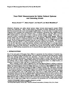
a. Borromean Rings 1 3 9665 48463 93877 52029 6614 4008 × 2888 8156

b. Trefoil Knot 1 1 3933 19929 38667 21479 2740 1393 × 1007 2839

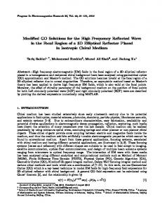
Figure 7. U22 in two cases of interesting topology: (a) complement of Borromoean rings (three unlinked but unseparable rings) and (b) complement of a trefoil knot. The current carrying regions are illustrated above the corresponding U22 and the tetrahedral FE mesh data in the table are for the complements of the respective ring and knot configurations.

Finite element-based algorithms to make cuts

235

of them is Poincar´e’s algorithm for computing the generators and relations of the fundamental group of a complex [35]. This construction is similar with the added constraint of preserving sparsity of the equations and reduction of the Poincar´e data into block U22 of ∂2T . Another relevant notion is that of the spine of a manifold [36]. In any case, an algorithm for finding {ζ1 , . . . , ζβ1 } can be summarized as follows: Algorithm 2 (Algorithm for 1-cocycle generator set) (1) Initialize: Set {ζ1 , . . . , ζβ1 } to be zero. (2) Maximal Tree: Construct a maximal spanning tree T on the 1skeleton of DK (3) Partition: Set ζi |T = 0 and partition ∂2T as in (46). (4) Forward Substitution: Forward substitute variables ζi |T (for all ζi these are the same variables) through U iteratively until the process halts. (5) U22 Nullbasis: Compute nullspace basis of U22 by a sparse null basis technique or by computing the Smith normal form. 5.4. The Size of U22 The process of partitioning ∂2T effectively retracts all the information about the topology of the mesh onto a 2-subcomplex of the mesh. The tree gives a retraction onto the 2-skeleton of K − ∂K, and the reduction by forward substitution is a retraction onto a 2-subcomplex ˜ has ˜ represented by U22 . In the dual mesh, the retraction, DK, K the same “homotopy type” as DK and hence the same (co)homology groups. For a sufficiently good maximal spanning tree (one that is, in some sense, short and fat), the number of 1-cells in U22 is the number of faces (of K) on S
a set of cuts plus additional surfaces which make any noncontractible loop on a cut contractible. Let N be some measure of the number of degrees of freedom per unit length ˘ 1 is linearly related to m0 in DK so that m0 is O(N 3 ). Note that m (Appendix A and [25]). Let k be the number of 1-cells in U22 , namely the number of free variables remaining in the reduced matrix. As the mesh is refined, k is on the order of the area of S
, that is O(N 2 ) or 2/3 O(m0 ). The complexity of an algorithm to compute the nullspace basis is O(m20 ) + O(k 3 ) in time and O(m0 ) + O(k 2 ) in storage, where 2/3 k is O(m0 ) so that the time complexity becomes O(m20 ) and space 4/3 complexity is O(m0 ). The overall time requirement for computing cuts is that of finding {ζ1 , . . . , ζβ1 } for each cut and β1 solutions of Laplace’s equation to find the nodal potential described in Section 3.

236

Gross and Kotiuga

6. SUMMARY AND CONCLUSIONS While Amp`ere’s law gives intuition about the role and nature of cuts, it sheds no light on their construction and computation. On the other hand, the algebraic structures of (co)homology theory are adequate for formulation of an algorithm for finding cuts on finite element meshes which are orientable, embedded submanifolds of the nonconducting region. The algorithm fits naturally into finite element theory. Starting with the connection matrix, cuts can always be found in O(m30 ) time and O(m20 ) storage. However, complexity can be improved 4/3 to O(m20 ) time and O(m0 ) storage by the algorithm outlined above. Moreover, the algorithm discussed in Section 5 preserves sparsity in the finite element matrices and thus does not adversely affect complexity in subsequent computation of a scalar potential with cuts. The speed of the algorithm can be further improved if one starts with a coarse mesh or information about the fundamental group π1 and its commutators [35]. It is clear that in the context of adaptive mesh refinement, cuts should be computed on a coarse mesh and then refined with the mesh since even the most coarse mesh contains all the information required for the topological computation. On the other hand, since the topological computation involves only integer arithmetic, computation on a fine mesh does not introduce rounding error. The algorithm has been implemented for tetrahedral and hexahedral finite element meshes. ACKNOWLEGMENT P. Gross gratefully acknowledges support received from the National Science Foundation, International Division, and Ikuo Saitoh of Hitachi Central Research Laboratory, Kokubunji, Japan, for constructive comments on this paper and in implementing the cuts algorithm. APPENDIX A. MESH-COUNTING ARITHMETIC A.1. The Euler Characteristic χ(R) The arguments of Table 1.2 and Section 5 rely on the Euler characteristic of a simplicial complex. This notion is best known in the context of the topology of polyhedra [2] and in electrical circuit theory, but in a more general form is useful for many arguments for finite element matrices [25]. Here we state the basic definition and theorem used in this paper. Proofs can be found in [28].

Finite element-based algorithms to make cuts

237

Let mi denote the number of i-simplexes in a tetrahedral finite element mesh K. The Euler characteristic χ(K) is defined as χ(K) =

3

(−1)i mi .

(A1)

i=0

The Euler characteristic is related to the ranks βi (K) of the homology groups of the simplicial complex of K as follows. Theorem. χ(K) =

3

(−1)i βi (K)

(A2)

i=0

The definition and theorem are the same for a cellular complex where mi denotes the number of i-cells in the complex, and while the statements above are given for a 3-complex, the definition and theorem are the same for an n-complex. A.2. The Details behind Table 1.2 Since a CG iteration involves one matrix-vector multiplication, two inner products and three vector updates, for a given interpolation scheme on a finite element mesh, the number of FLOPS per CG iteration is [25] F = 5D + X

(A3)

where D is the number of degrees of freedom and X is the number of nonzero entries in the stiffness matrix. For the scalar Laplace equation, we can use the notation of Table 1.2 and write: F0s = 5D0s + X0s

(A4)

where X0s

D0s = m0 . = m0 + 2m1

(A5)

and mi , 0 ≤ i ≤ 3 are the number of i-simplexes in the mesh. Similarly, let ni be the number of i-simplexes in the boundary of the mesh. Since we have the linear relations [23] m1 = m0 + m3 + n0 − 3χ(R) m2 = 2m3 + n0 − 2χ(R)

(A6)

238

Gross and Kotiuga

equation (A4) can be rewritten as F0s = 8m0 + 2m3 + 2n0 − 6χ(R).

(A7)

For nodal interpolation of three-component vectors, F0 = 5D0 + X0

(A8)

D0 = 3D0s . X0 = 3(3X0s )

(A9)

where

Using equations (A6) and (A5), equation (A9) can be substituted into (A8) to yield F0 = 42m0 + 18m3 + 18n0 − 54χ(R)

(A10)

Similarly [25], for edge interpolation of vectors, we can write F1 = 5D1 + X1

(A11)

where, by [25] D1 = m1 and X1 = m1 + 2(3m2 ) + 6m3 .

(A12)

Then, via equation (A6) we have F1 = 6m0 + 24m3 + 12n0 − 30χ(R).

(A13)

Assuming that hexahedral meshes have, on average, as many nodes as elements, a useful heuristic is m3 = km0 where k = 5 or 6 (depending on whether hexahedra are divided into 5 or 6 tetrahedra). So, comparing (A10) and (A13) to (A7), one finds that in the limit, as the mesh is refined (m0 → ∞)  F0 7.5 k = 6 (A14) = 7.6 k = 5 F0s and F1 = F0s



10.7 k = 6 9.7 k = 5

(A15)

This is the bottom line of Table 1.2. The top line of the table is derived similarly by using equations (A5), (A9), and (A12), then using (A6), forming ratios, and letting m0 → ∞ in the ratios. See also [33] for numerical evidence.

Finite element-based algorithms to make cuts

239

APPENDIX B. WHY FINITE ELEMENT ANALYSIS OF MAGNETIC FIELDS IS EASY ONCE CUTS ARE IN HAND Given cuts, we can view the computation of magnetic scalar potentials in multiply-connected regions as follows. For a real-valued potential ψ we have  1 µ grad ψ · grad ψ dV. (B1) F (ψ) = 2 R Given that cuts are orientable surfaces [20] and thus have a wellnˆ ψ+

ψ−

Figure B1. ψ + and ψ − on each side of the cut surface and the normal to the cut. defined surface normal, let ψ + (ψ − ) be the value of the potential on the “positive” (“minus”) side of a cut (denoted by Si+ (Si− )), with respect to a normal defined on the cut surface as shown in Figure B1. Let ψB denote the potential on the boundary of the region. Then (B1) is subject to ψ + − ψ − = Ji on Si ψ = ψB given on ∂R.

(B2)

Here {Si }, 1 ≤ i ≤ β1 (R) generate H2 (R, ∂R), Si is built out of faces of the finite element mesh and the jumps Ji are determined by Amp`ere’s Law (Figure 1). Using barycentric coordinates, {λi }, 1 ≤ i ≤ 4, and interpolating ψ linearly on the vertices of the kth tetrahedron, k

ψ =

4

λn ψnk

(B3)

n=1

where ψnk represents the discretisation of ψ. Then the “assembled problem” is 3

1

l l ψm Kmn ψnl . 2

m

F (ψ) =

4

4

l=1 m=1 n=1

(B4)

240

Gross and Kotiuga

where the element stiffness matrix is now weighted by the element permeability µ. Define β1 (R) indicator functions {Ip }, 1 ≤ p ≤ β1 (R), as follows:  1 if mth node of lth tetrahedron ∈ Sp+ Ip (m, l) = . (B5) 0 otherwise Connecting the solution across tetrahedra and allowing for jumps in the scalar potential across cuts, ψnl

=

m0



β1 (R) l Cni ui

+

Jp Ip (n, l)

(B6)

p=1

i=1

This is equivalent to equation (26), but in (B6) (interelement) jumps in the potential are across cuts. Then, putting (B6) into (B4), we can write   β1 m3

m0 4 4





1 l l  Cmi ui + Jp Ip (m, l) Kmn · F (ui , Jk ) = 2 p=1 i=1 l=1 m=1 n=1   β1 m0



l  Cnj uj + Jq Iq (n, l) . (B7) q=1

j=1

Separating constant, linear, and quadratic terms in ui , and using (32), we have   β1 m0 m0

m0



1 ui uj Kij + ui  Jp fpi  + constants (B8) F (ui , Jk ) = 2 i=1 j=1

i=1

p=1

where, in analogy to equation (33), fpi =

m3

4

4

l l Cmi Kmn Ip (n, l).

(B9)

l=1 m=1 n=1

Then the discretized Euler-Lagrange equation for the functional (B1) subject to (B2) is Ku = −

β1

Jp fp

(B10)

p=1

where the elements of Kij , given by (32), are now weighted by µ, and fp is the vector with entries {fpi }. This equation is analogous to equation (31).

Finite element-based algorithms to make cuts

241

Table of Notation βp (R) δji ∂ ∂T ∂˘ θ θji {λi } µ π σip ψ ψ + (ψ − ) χ ζji B Bp Bp cp i Cjk Cp d DK F, G F0s F0 F1 fp f∗ Ip (m, l) Jji ∈ Z Jj ∈ R

pth Betti number = Rank Hp (R). Kronecker delta; 1 if i = j, 0 otherwise. Boundary operator. Coboundary operator. Boundary operator on dual mesh. Normalized angle of f : R −→ S 1 . θ discretized on nodes of unassembled mesh. Barycentric coordinates, 1 ≤ i ≤ 4. Magnetic permeability. Circumference to radius ratio of a circle. ith p-simplex in a triangulation of R. Magnetic scalar potential. Value of ψ on plus (minus) side of a cut. Euler characteristic (see appendix 1). jth 1-cocycle on dual mesh, indexed on 1-cells of DK: 1 ≤ i ≤ m ˘ 1. Magnetic flux density vector. p-coboundary. p-boundary. p-cochain. Connection matrix, 1 ≤ i ≤ m3 , 1 ≤ j ≤ 4, 1 ≤ k ≤ m0 . pth chain group. Coboundary operator. Dual cell complex of simplicial complex K. Spaces of vector fields with elements F and G, resp.. # FLOPs per CG iteration for node-based interpolation of scalar Laplace equation. # FLOPs per CG iteration for node-based vector interpolation. # FLOPs per CG iteration for edge-based vector interpolation. “forcing function” associated with the pth cut (a vector with entries fpi ). Pullback of f . Indicator function, 1 ≤ p ≤ β1 (R), 1 ≤ m ≤ 4, 1 ≤ l ≤ m3 . Nodal jumps on each element, 1 ≤ i ≤ m3 , 1 ≤ j ≤ 4. Jump across ith cut.

242

H H p (R; Z) Hp (R; Z) H p (R, ∂R; Z) Hp (R, ∂R; Z) K k Kmn mp m ˘p np O(nα ) P R S Sq S1 uk X0s X0 X1 z zp zp [A, B]

Gross and Kotiuga

Magnetic field intensity. pth cohomology group of R with coefficients in Z. pth homology group of R, coefficients in Z. pth cohomology group of R relative to ∂R, coefficients in Z. pth homology group of R relative to ∂R, coefficients in Z. Simplicial complex. Stiffness matrix, 1 ≤ m, n ≤ 4, 1 ≤ k ≤ m3 . Number of p-simplexes in a triangulation of R. Number of p-cells in dual complex. Number of p-simplexes in a triangulation of ∂R. Order nα . Period matrix, equation (21). Region in R3 , free of conduction currents, where the field is sought. Surface. qth cut. Unit circle, S 1 = {p ∈ C | |p| = 1}. Nodal potential, 1 ≤ k ≤ m0 . # nonzero entries in stiffness matrix for node-based scalar interpolation. # nonzero entries in stiffness matrix for node-based vector interpolation. # nonzero entries in stiffness matrix for edge-based vector interpolation. Complex conjugate of z. p-cocycle. p-cycle. Homotopy classes of maps f : A → B.

REFERENCES 1. Adkins, W. A. and S. H. Weintraub, Algebra: An Approach via Module Theory, 307–327, Springer-Verlag, New York, 1992. 2. Armstrong, M., Basic Topology, Springer-Verlag, New York, 1983. 3. Balabanian, N. and T. A. Bickart, Electrical Network Theory, 80, John Wiley and Sons, New York, 1969. 4. Bamberg, P. and S. Sternberg, A Course in Mathematics for Students of Physics: 2, Ch. 12, Cambridge U. Press, NY, 1990. 5. Bossavit, A., A. Vourdas, and K. J. Binns, “Magnetostatics with scalar potentials in multiply connected regions,” IEE Proc. A,

Finite element-based algorithms to make cuts

243

Vol. 136, 260–261, 1989. 6. Bott, R. and L. W. Tu, Differential Forms in Algebraic Topology, 40–42, 51, 234, 258, 240, Springer-Verlag, New York, 1982. 7. Brown, M. L., “Scalar potentials in multiply connected regions,” Int. J. Numer. Meth. Eng., Vol. 20, 665–680, 1984. 8. Cohen, H., A Course in Computational Algebraic Number Theory, Springer-Verlag, New York, 1993. 9. Coleman, T. F., A. Edenbrandt, and J. R. Gilbert, “Predicting fill for sparse orthogonal factorization,” Journal of the Association for Computing Machinery, Vol. 33, 517–532, 1986. 10. Croom, F. H., Basic Concepts of Algebraic Topology, Chaps. 2, 7.3, 4.5, Springer-Verlag, New York, 1978. 11. Deschamps, G. A., “Electromagnetics and differential forms,” IEEE Proc., Vol. 69, 676–696, 1981. 12. Greenberg, M. J. and J. R. Harper, Algebraic Topology, 235, 63–66 Benjamin/Cummings, Reading, MA, 1981. 13. Gross, P. W., “The commutator subgroup of the first homotopy group and cuts for scalar potentials in multiply connected regions,” Master’s thesis, Dept. of Biomed. Eng., Boston U., September 1993. 14. Gross, P. W. and P. R. Kotiuga, “Data structures for geometric and topological aspects of finite element algorithms,” this volume. 15. Gross, P. W. and P. R. Kotiuga, “A challenge for magnetic scalar potential formulations of 3-d eddy current problems: Multiply connected cuts in multiply connected regions which necessarily leave the cut complement multiply connected,” Electric and Magnetic Fields: From Numerical Models to Industrial Applications, A. Nicolet and R. Belmans (eds.), Plenum, 1–20, New York, 1995. Proc. of the Second Int. Workshop on Electric and Magnetic Fields. 16. Guillemin, V. and A. Pollack, Differential Topology, 21, PrenticeHall, Englewood Cliffs, New Jersey, 1974. 17. Gunning, R. C. and H. Rossi, Analytic Functions of Several Complex Variables, Prentice-Hall, Englewood Cliffs, N.J., 1965. 18. Harrold, C. S. and J. Simkin, “Cutting multiply connected domains,” IEEE Trans. Magn., Vol. 21, 2495–2498, 1985. 19. Kotiuga, P. R., “Hodge decompositions and computational electromagnetics,” Ph.D. thesis, McGill University, Montreal, 1984. 20. Kotiuga, P. R., “On making cuts for magnetic scalar potentials in multiply connected regions,” J. Appl. Phys., Vol. 61, 3916–3918,

244

Gross and Kotiuga

1987. 21. Kotiuga, P. R., “An algorithm to make cuts for scalar potentials in tetrahedral meshes based on the finite element method,” IEEE Trans. Magn., Vol. 25, 4129–4131, 1989. 22. Kotiuga, P. R., “Topological considerations in coupling scalar potentials to stream functions describing surface currents,” IEEE Trans. Magn., Vol. 25, 2925–2927, 1989. 23. Kotiuga, P. R., “Analysis of finite-element matrices arising from discretizations of helicity functionals,” J. Appl. Phys., Vol. 67, 5815–5817, 1990. 24. Kotiuga, P. R., “Topological duality in three-dimensional eddycurrent problems and its role in computer-aided problem formulation,” J. Appl. Phys., Vol. 67, 4717–4719, 1990. 25. Kotiuga, P. R., “Essential arithmetic for evaluating three dimensional vector finite element interpolation schemes,” IEEE Trans. Magn., Vol. 27, 5208–5210, 1991. 26. Kotiuga, P. R., A. Vourdas, and K. J. Binns, “Magnetostatics with scalar potentials in multiply connected regions,” IEE Proc. A, Vol. 137, 231–232, 1990. 27. Maxwell, J. C., A Treatise on Electricity and Magnetism (1891), Chap. 1, Art. 18–22, Dover, New York, 1954. 28. Munkres, J. R., Elements of Algebraic Topology, 377–380, Addison-Wesley, Reading, MA, 1984. 29. Murphy, A., “Implementation of a finite element based algorithm to make cuts for magnetic scalar potentials,” Master’s thesis, Dept. of ECS Eng., Boston U., 1991. 30. Pothen, A. and C.-J. Fan, “Computing the block triangular form of a sparse matrix,” ACM Transactions on Mathematical Software, Vol. 16, 303–324, 1990. 31. Ren, Z. and A. Razek, “Boundary edge elements and spanning tree technique in three-dimensional electromagnetic field computation,” Int. J. Num. Meth. Eng., Vol. 36, 2877–2893, 1993. 32. Rotman, J. J., An Introduction to Algebraic Topology, SpringerVerlag, NY, 1988. 33. Saitoh, I., “Perturbed H-method without the Lagrange multiplier for three dimensional nonlinear magnetostatic problems,” IEEE Trans. Magn., Vol. 30, 4302–4304, 1994. 34. Silvester, P. and R. Ferrari, Finite Elements for Electrical Engineers, 2nd Edition, Cambridge U. Press, NY, 1990. 35. Stillwell, J., Classical Topology and Combinatorial Group Theory, Second Edition, Ch. 3,4, Springer-Verlag, NY, 1993.

Finite element-based algorithms to make cuts

245

36. Thurston, W. P., Three-Dimensional Geometry and Topology, Princeton University Press, Princeton, New Jersey, 1997. 37. Vourdas, A. and K. J. Binns, “Magnetostatics with scalar potentials in multiply connected regions,” IEE Proc. A, Vol. 136, 49–54, 1989.