guide containing a plug of lossy magnetic material are compared with the analytic solution. The alternative dual variables are successively employed, treated as ...
SCIENCE
Finite-element modelling of high-frequency electromagnetic problems with material discontinuities R.L. Ferrari, MA, BSc, CEng, MlEE R.L. Naidu, BSc, PhD
Indexing terms: Electromagnetics, Finite-element modelling, Eigenvalues
Abstract: A weighted residual formulation, suitable for finite-element application, is given for the general high-frequency time-harmonic electromagnetic problem presented by a lossy anisotropic inhomogeneous boundary driven linear system. Either of the dual field vectors H or E may be chosen as the working variable. New light is thrown on the difficulties arising in finite-element analysis when components of the working variable are discontinuous owing to sharp jumps in material properties. The latter are shown to represent ‘natural’ boundaries not specifically requiring any constraint. The modification of the formulation applying to the eigenproblem of an axially uniform waveguide is presented. The equivalence of the Galerkin option of the formulation used in the paper and the corresponding variational approach is discussed. Some finiteelement numerical results relating to the analytically soluble problem of a waveguide with an axial discontinuity in material property are presented, confirming the predictions made and demonstrating the practical possibility of solving highfrequency problems by the finite-element method successively with dual working variables. 1
Introduction
Solution of low-frequency electromagnetic problems by the finite element method is by now a well established procedure, and the corresponding software packages are widely available [l]. Standard approaches employ a single scalar potential variable wherever possible, but require a vector variable, commonly chosen to be the vector magnetic potential A , for eddy current regions. The finite element formulations are worked out either from variational principles [2] or using the Galerkin option of the weighted residual method [ 3 , 41. Either method is ordinarily expected to give the same result. Applied to high frequency problems (that is for cases where the inclusion of displacement current is obligatory Paper 7492A (S8), first received 4th January and in revised form 25th June 1990 MI. Ferrari is, and Dr. Naidu was formerly, with the Department of Engineering, University of Cambridge, Trumpington Street, Cambridge CB2 lPZ, United Kingdom Dr. Naidu is now with the Department of Civil Engineering, University of Malaya, Kuala Lumpur 22-1 1, Malaysia
IEE PROCEEDINGS. Vol. 137, Pt A, N o 6 , NOVEMBER 1990
and where device dimensions approach the same order as oscillation wavelengths) the finite element method is much less well developed. In general at least two independent space and time-varying variables, such as the longitudinal components of both electric and magnetic fields inside a waveguide, must be used. For truly threedimensional situations, or in cases where anisotropic material is present, there is much to be said for employing a three-component vector and for choosing this to be a field variable, either E or H, rather than a vector potential. The common approach for high-frequency finiteelement vector-variable formulations is via a variational route, both for three-dimensional problems [ 5 ] and for the special two-dimensional case represented by an axially uniform waveguide [6, 71. In the present work it is found that the treatment applicable to material discontinuities follows very conveniently from a weighted residual analysis. However Zienkiewicz and Taylor [SI point out that, in cases where the Euler equations of the variational principle coincide with the governing equations used in setting up a Galerkin weighted residual solution, the latter corresponds precisely to the variational result. For the particular case discussed here, equivalence of the Galerkin and variational methods does in fact hold. A weighted residual formulation of the general highfrequency, time-harmonic electromagnetic problem is presented following the general principles indicated by Zienkiewicz and Taylor [SI for a scalar variable and by Biddlecombe et al. [4] for vector potential in the lowfrequency eddy current problem. The full threedimensional problem involving lossy and anisotropic materials is examined, employing a field-vector working variable. The position with regard to solutions obtained in cases where the component of the field-variable normal to a material interface becomes discontinuous is clarified. The current standard practice, when applying the finite element method to high frequency device problems involving material discontinuities, is to avoid the choice of a working variable which has discontinuous components. Thus the H-variable is invariably selected when analysing waveguides with a dielectric inhomogeneity [6, 7, 12, 131; normally no attempt is made at exploiting use of the dual variable E or of gaining the computational advantage which might result in performing both of the dual calculations. It is shown here that material interfaces behave as ‘natural’ boundaries requiring no particular constraint but only adequate discretisation to allow the field discontinuity to be modelled to sufficient accuracy. A formulation for extracting the 313
eigensolutions of the two-dimensional lossy waveguide problem is then developed from the essentially threedimensional weighted residual procedure applying to boundary driven configurations. The Galerkin weighted residual option of the general procedure here corresponds with the variational formulations [SI and [7]. Some finite element numerical results relating to the 'benchmark' problem of a short-circuit rectangular waveguide containing a plug of lossy magnetic material are compared with the analytic solution. The alternative dual variables are successively employed, treated as if they were continuous at every finite element node, however ensuring that the discretisation locally is sufficiently fine to accommodate a sharp spatial field variation. Excellent agreement with theory is obtained for both field and global parameters, even though there was nominally a discontinuity in one component of the H-variable at the material interface. 2
Fundamental equations for linear time-harmonic problems
Consider Maxwell's equations in their complex phasor form applicable to steady-state oscillations at frequency o in a linear system: V x E = -jwp 0P.H (1) V x H = jws,e,E (2) Because a linear conductivity is assumed, the customary term in eqn. 2 representing electric current may be omitted. Instead, the effects of conduction current are included by allowing e, to be complex. Magnetic losses are correspondingly accounted for in a linear model by means of complex p,. In addition, anisotropy may be taken into account, in which case the constitutive parameters assume a tensor form depending on the exact nature of the material concerned (see Reference 9 for a discussion of the representation of general anisotropic dielectrics, ferrites and plasmas). A problem domain bounded by a closed surface is considered. In general the bounding surface may comprise any or all of the following: an electric wall representing a surface on which n x E = 0; a magnetic wall on which n x H = 0; or coupling ports over which a transverse field, either n x E = E, or n x H = H,, is prescribed. The so-called electric and magnetic walls arise principally from perfect conductors and infinitely permeable magnetic boundaries respectively, but can also be established as a result of symmetry. In general, many practical high-frequency electromagnetic problems with external field excitation, for instance n-port waveguide junctions and cavity configurations, can be specified in terms of such enveloping boundary constraints. Stratton, on pages 485488 of Reference 10,shows that, in order to obtain a unique field solution inside R, it is necessary only to specify either transverse E or transverse H over the coupling surfaces S , . Eqns. 1 and 2 may be combined to give either V x e,-'V x H - k2p,H = 0
(3)
or V xp';'V x E - k 2 e , E = 0 where
(4)
kZ = o z p 0c0 (5) Suppose the problem space R contains discontinuities of permeability and/or permittivity, corresponding to interfaces between differing material media. In systems, such 314
as here, deemed to be charge- and current-free through the device of assuming complex tensor constitutive constants pop, and E ~ E , , it is well known that tangential components H, and E, of the field intensities must always remain continuous on passing through any such interface, whereas the normal component of these vectors, H. and En, will be discontinuous insofar as the requirement that continuity of the corresponding normal components of B = p0 p, H and D = eo e, E has to be met. Stratton, on page 34 of Reference 10, remarks that closer examination of these rules reveals that their strict derivation, as a consequence of the axiom that Maxwell's equations apply universally, requires consideration of the limiting case of a physical model where the material constants vary sharply but continuously from one medium to another. Furthermore, for solving practical problems, Plonsey and Collin [l 11, page 320, show that it is merely necessary to establish the continuity of both H, and E, at any interface, without specific reference to the continuity of B, and D , , provided it is ensured that H and E together satisfy Maxwell's equations (eqns. 1 and 2) in the continuum on either side of the boundary. The required continuity of Bn and D, then follows automatically. Consider a spatially discretised field solution, worked say in terms of the magnetic vector variable H, in which eqn. 3, representing Maxwell's curl equations, is satisfied at the general mesh point by means of a numerical process. Furthermore, suppose that it is ensured that continuity of both tangential components of H and E = e,-'V x H/jwcO is maintained across all material interfaces, the latter condition corresponding to a numerical implementation of the curl operator acting upon the discretised H. With an adequately fine mesh it would seem likely that the issue as to whether Hn displays precisely the idealised discontinuity behaviour need not be faced; a numerical result that reproduces the spatial step in Hnas a graded numerical approximation is quite acceptable. In such a case, it may be more convenient to treat all components of H as being continuous. It will be shown that indeed such a procedure is 'natural' to the vector weighted residual process for solving the general electromagnetic problem defined here. It is to be expected that the numerical value returned at any node where there is an ideally discontinuous field component will be an appropriate average of the discontinuity field. Such a numerical phenomenon is not unknown in the field of computational analysis; in numerically inverting the Fourier transform of a step function an average value is always returned at the step discontinuity itself, whilst the sharpness of the step reproduction is dependent on the fineness of discretisation chosen. 3
General weighted residuals procedure
The weighted residual analysis set out here is an extension of that given by Biddlecombe et al. [4] applying to the vector potential A in eddy current problems; the extension concerns treatment of cases where abrupt changes of materials occur. The weighted residual procedure followed is spelt out fairly fully for convenience. The analysis is restricted to considering eqn. 3 in detail, equivalent to choosing H as the working variable. The procedure required to use the alternative starting point of eqn. 4, working with the E-vector, follows trivially. When considering, as here, a magnetic variable, the constraint applicable at an electric wall, namely the homogeneous Dirichlet condition of vanishing tangential electric field, IEL. PROCEEDINGS, Vol. 137, Pr. A, N o . 6, N O V E M B E R 1990
may be taken from eqn. (2) as E,-'V x H=O
n x
To establish the weighted residual procedure applying to a general three-dimensional problem domain R containing abrupt changes in E, and/or p,, the geometry of Fig. 1
I
Schematic representation of a problem space with a material Fig. 1 discontinuity
--
couphng surface s,
I-rm ~
ekClrlc wall S E magnetic wall S , material interface S,
Lw.[V x (E;'V x H)] dR
is considered. For simplicity, R will be supposed to be made up from just two regions, R, and R, , separated by an interface surface S, at which the abrupt change occurs. The problem exterior boundary is made up from a magnetic wall s,, an electric wall S E and a coupling surface S,, where at each surface the field H must satisfy appropriate boundary conditions. The trial H-variable used here (but not necessarily its space derivatives) will be assumed continuous throughout R, so that tangential H on S I is automatically continuous. Implicit continuity of tangential E is obtained by requiring n x E,-'V x H to be continuous on S,. The assumption embodied in Fig. 1, that R, is a single, simply connected region lying wholly inside the problem boundary S , so that S I happens to be a simple closed surface, simplifies the analysis to be given here. However, there is no difficulty in extending the argument to relate to more complicated topologies; the end result is the same. Define weighted residual terms as follows: =
JI,
W * ( V x E,'V x H - k'p,H) dR
(7)
E;'V x H - kZp,,H)dR
(8)
R,
= L,W.(V x
Rs
=
LI,
W,.(n x H ) d S +
+
RI
s,,
WE*(n x E;'V x H ) dS
W, .n x (H - H,) dS
W , * n x [(E:'V
=
H if the residual R = R I + R , + R , + RI vanishes for all sets { W, W,, W E ,W , , W , } of the arbitrary weighting functions. The general weighted residual method of obtaining an approximate solution to a problem such as is considered here proceeds by choosing some reasonable form for a 'trial' solution, here the function H(r), embodying any number of undetermined parameters. An appropriate number of different sets of the arbitrary weighting functions are chosen and are notionally substituted in turn into eqns. 7-10. If the integrations indicated were to be performed and the residual R , associated with every arbitrary set of weights, { W . . W , } , put to zero, then equations would be set up so as to allow the undetermined parameters to be solved for. Within the limitations of the function-space chosen for the trial H, a best estimate of the exact solution satisfying the continuum equation (eqn. 3) and its boundary constraints would then be achieved. However, as in the eddy current analysis [4], before attempting to carry out this process an integration by parts using the general vector relationship
(9)
x H), - ( E : ' V x H),] dS (10)
SI
where the weights W, W,, . . ., W , , the field H a n d derivatives of the latter are suitably continuous to allow the integrations of eqns. 7-10 to proceed. The weighting term expressed by eqn. 10 relates to the required continuity of tangential E at the material interface S,; the normal to S,, n, is taken as pointing from R I into 0,. It is seen that R , and R , vanish if the external boundary constraints on S and the interface constraints on S I , respectively, are met. Thus eqn. 3 and its associated boundary/interface constraints must have been satisfied by the trial function IEE PROCEEDINGS, Vol. 137, Pt. A , N o 6 , N O V E M B E R 1990
=i
( V x W ) .[E;'V x
dR
-kWX(EL'VXH)-ndS
(11)
is applied to the subregions R, and 0,. This reduces the order of differentiation in the weighted residual constructions (eqns. 7 and 8), so that the continuity requirements of H and W alike become CO,instead of the more stringent imposition upon H placed by the original weighting expressions (see Reference 8, chapter 7). Quite a substantial simplification of the integral expression for R is also obtained from performing such an integration by parts and placing the following restrictions upon H a n d W : (i) The trial function H and the weight Ware assumed to be CO-continuousfunctions of position within R. (ii) The trial H is restricted to vector functions whose transverse components on S, are specified as H,, satisfying the inhomogeneous Direchlet condition there. Because of the properties of the vector product with n it is not seen from eqn. 9 that the normal components of H on S , need not be given. (iii) The trial H is restricted such that n x H = 0 on S,. As in (ii), the imposition of the homogeneous Dirichlet boundary condition here also merely requires that attention be paid to the transverse components of H. (iv) The weighting functions W are restricted to those making n x W vanish on both the inhomogeneous and homogeneous Dirichlet boundaries, here S, and S, . (v) Without loss of generality, choose W E= - W on the homogeneous Neumann boundary S E . After some straightforward but lengthy algebra manipulating exprs. 7-9, following the standard pattern for electromagnetics weighted-residual analysis [3, 41, the simplification below is arrived at for the sum of the corresponding three terms of the overall residual : RI =
+ R , + Rs j [ ( V x W).(E,'V -
!",
X
H ) - k Z W . @ , H ) ] dS2
W x [(E;'V x H), - (E; 'V x H),]
.n dS
(12) 315
Now choose (without loss of generality) W , = - W on S, and substitute this choice into expr. 10 for R,. Applying the rules of vector algebra concerning permutation of the order of operations in vector triple products and then forming the sum R = R , + R , + R , + R , , there is cancellation of the integrals taken over S, such that adding exprs. 10 and 12 gives R=
J1,
[ ( V X W).(e,'VxH)-k'W.(/c,H)]dR
(13)
to be forced to zero by the proper choice of the trial function H . Setting to zero the expression given in eqn. 13 thus forms the basis for a weighted residual solution of the electromagnetic problem described here. It should be noted that expr. 13 is precisely the same as would arise without a discontinuity at S,. Since the classical conditions [IO, 111 required to ensure a unique field solution throughout the composite region have, within the limitations of the trial function for H , been satisfied, it may be concluded that the interface S , represents a 'natural' boundary which needs no constraint. No precise information has been extracted concerning the finite-element field values expected precisely on the discontinuity boundary. However it is seen that, with adequate discretisation, on either side of the boundary, as elsewhere, a correct solution to Maxwell's equations can be approached numerically as closely as is desired. 4
Weighted residual formulation for uniform waveguides
The preceding analysis is not immediately applicable to the problem of determining the modes of a uniform waveguide, because the transverse field distribution over the waveguide cross-section is unknown, whereas the residual eqn. 13 has been derived on the basis that known boundary constraints apply over the whole closed surface defining the problem region. However, consider a waveguide, with a constant but possibly inhomogeneous cross-section, having its axis aligned with the z-direction. For a given waveguide mode progressing in the +zdirection, the phasor magnetic field may be written H ( x , Y , 4 = H o b , y ) exp (-jPz) (14) The problem now presented consists formally of finding complex eigenvectors H o and eigenvalues 8,given real k, corresponding to a general lossy configuration involving complex p? and E , . Let PI be a notional input plane at z = 0 where, for a waveguide carrying the mode (eqn. 14) H = Hob, Y) (15) Similarly let P , be a corresponding output plane at z = d, where H = Ho(x, Y ) exp (-JBd) (16) Then the composite closed surface S = S E + S , + P , + P , may be taken to define a problem region R, where SE and S , are natural boundaries having the same significance as before. A weighted residual for the problem may be written as R
=
b
W . ( V x E,-,V x H
+ b M W M.(n x
k2p,H) d R
H ) dS
+ b , W E . ( n x E;'V 316
-
x H) dS
(17)
It has been established already that internal boundaries corresponding to abrupt changes of material property represent natural boundaries, requiring no corresponding specific weighting term. However the residual eqn. 17 also omits any terms corresponding to SI and S,, the open ends of the waveguide. Instead it is required that eqn. 14 shall be satisfied everywhere throughout R and on S , and S, . The same manipulations are performed as in the general three-dimensional analysis, except that the transverse field components on S, and S , (corresponding to S,) necessarily remain unspecified. Now, with the trial H , restricted to functions meeting the magnetic wall homogeneous Dirichlet condition, and with the weighting functions constrained also to vanish on such a wall, the residual eqn. 17 reduces to
R
=
b
[(V x W).(E,-'V x H) - k 2 W . ( / c , H ) ]d R
-
b , W x (EL'V x H)] ' n l dS
-
121W x (E,1V x H)]
a n ,
dS
(18)
The normals to S , and S,, n1 and n , , respectively, are equal and opposite. Thus if now W = W,,(x, y ) exp ( + j g z ) is chosen, then, because of the requirement that H shall be the positive-travelling single waveguide mode (eqn. 16) associated with the wave factor exp (-jbz), it is seen that the last two integrals in eqn. 18 cancel one another and the rest of the terms in that expression are constant with z. Denoting V * ) x as the operator such that
V(*' x F
I LX
i
I
a/Sx 3/31> _+jD (19) F, :z where F is any vector, it is seen that the residual eqn. 18 may now be cast into the form R
=
=
I,
[(V(" x W , ) * ( E , - ' V ( - )x H o ) - k Z WO
.p , Ho] dx d y
(20)
where S, is any cross-section of the waveguide normal to its axis, dependent only on the transverse co-ordinates x and y. Once again a sufficient number of different weighting functions WOmust be chosen in order to solve for the unknown parameters defining the trial function H , . However in contrast with the previous problem, which concerned specific excitation at coupling surfaces, here the matrix equations set up take the form of an eigenvalue problem. Given a frequency k, there ensues a set of eigenvalues Ho(x, y ) together with an associated set of eigenvalues P. In practice, a more tractable numerical analysis is expected to follow if, as is quite permissible, 8 is specified and k is treated as being the unknown eigenvalue. 5
Galerkin and variational finite-element procedures
Galerkin's method represents a special case of the weighted residual procedure wherein the weighting functions are chosen from the specific function space used to form the trial solution. When the Euler equations corresponding to a variational approach are the same as the equations used to set up Galerkin's solution, it may be assumed that the two methods are exactly equivalent [SI. I E E P R O C M D I N G S , V o l . 137, Pi A , No. 6, N O V E M B E R 1990
When setting up finite element equations, investigators in numerical electromagnetics, e.g. References 2-7, tend to select one of the above methods according to individual taste without concerning themselves with the other. Here, with a field-vector variable, the Galerkin procedure commences routinely with the representation of the trial function separately in each finite element R, in terms of nodal vector unknowns Heisuch that He = Hei Nei(r) where Nci(r)is a scalar shape function
(21)
[SI
such that
Nei(rej)= 6ij
(22)
and dij is the Kroenecker delta. The Galerkin procedure continues with the construction of vector weighting functions from the scalar shape functions, three for each node corresponding to the three unknown components at each general node: W i= (1, 0, O)Nei(r) W i= (0, 1, O)Nei(r)
W i = (0,0, l)Nei(r) (23) There is an understanding that outside the element Re, which itself may be composite because a node i is common to two or more subelements, the weighting vectors are identically zero. Because of the basic property of the shape functions (eqn. 22), these weighting functions also vanish at the element boundary. Thus the requirement 3(i) that every W shall be CO-continuousthroughout the whole of R is satisfied. In order to accommodate nodes lying on a Dirichlet surface, either S , or S , , suppose that such a surface has unit normal vector no. The requirement 3(iv) is that n, x W shall vanish. This will automatically occur if just one weighting vector W = noNei(r) associated with a given node is selected. This is a sufficient number, since because of the nature of the Dirichlet constraint to be imposed on the trial function, only one independent vector component variable is now left free. At the same time this constraint
n,xH=H, (25) where Hc is prescribed (on S,) or vanishes (on S,) enables the vector variable H at a Dirichlet node to be expressed in terms of a single scalar unknown. The prescription embodied in eqn. 21 combined with the choice of weights as above is clearly sufficient to set up the matrix equations that determine, by substitution into either eqn. 1 3 or eqn. 20, matrix equations that define the unknown vector set Hei. In a variational approach to problems such as are considered here, the stationarity of the functional
F, =
b
[V x HE,-’V x H
~
k 2 H p , f l dR
(26)
is exploited [5, 71. The first variation of F , vanishes for the solution sought provided the trial function H is restricted in the same way as described for the weighted residual process, namely that it shall conform to Dirichlet boundary constraints wherever these apply and that it shall be continuous throughout R. (The position with respect to material discontinuities that would make the working variable nominally discontinuous has not previously been clarified.) For a finite-element process, the trial vector function H is again expressed in terms of shape functions as in eqn. 21. The proposition that making the functional (eqn. 26) stationary with respect to the trial H is equivalent to the Galerkin process [SI is IEE PROCEEDINGS, Vol. 137, Pt. A, No. 6 , N O V E M B E R 1990
readily verified in detail, both for the three-dimensional case covered in Reference 5 and for the eigenvalue problem [7]. Thus provided suitable discretisation is chosen, there is no reason why the finite-element programs used in References 5, 6, 7, 12 and 13 should not be applied to systems where the working vector variable nominally has discontinuous components. 6
Numerical verification
A finite element field solver for high-frequency timeharmonic problems involving linear, isotropic media has previously been reported on [5, 12, 131. This solver returns interior nodal values of a vector field, either H or E to choice, corresponding to eqn. 3 or eqn. 4, respectively, in cases where Stratton’s boundary conditions (see Section 2) have been properly specified. The program nominally proceeds by means of a finite-element realisation of the stationarity of either the functional F , , defined by eqn. 26 (but here with scalar relative constitutive parameters p, and E, corresponding to the restriction to isotropic materials), or of an electric field dual F E . However, as has been explained, the programming and computation are precisely the same as would have arisen from the Galerkin method. The solver requires the problem-space to be discretised into ‘superelements’ which it then subdivides automatically into tetrahedra of order 1 4 . Properties corresponding either to air, a lossy magnetic material or a lossy dielectric are assigned to each superelement; the solver works in terms of a complex vector variable evaluated at each of the finite element nodes. In the previous investigations with this solver, as in other work [6, 71, cases where the working variable becomes discontinuous have always been avoided; consequently no results have been recorded comparing dual solutions. Here we report on the testing of the proposition that such a solver may be used for geometries where there are spatial discontinuities of p, and/or E,, without making special provision for any corresponding discontinuity of the vector working variable. At the same time it is demonstrated that solving a given problem in both of its dual forms is possible; under some circumstances the freedom to work successively in both dual modes of computation could represent a valuable aid to achieving accuracy. The configuration chosen for test purposes was a length of rectangular waveguide terminated with a block of lossy magnetic material followed by a short circuit (Fig. 2) and carrying the dominant TE,, mode. Such a open-end TEIO excitation
lossy plug
i
pr=pre -1pr
c=lm
:0333m 0
a:2m Fig. 2 Rectangular waveguide containing a lossy plug The dimensions shown were fed in as computer data in metres, but normalisation IS implied
317
geometry has a closed form analytical solution, and so it represents a very suitable 'benchmark' problem. The waveguide dimensions and corresponding frequency range appropriate to the waveguide mode selected may /\
F , = j c o s , ~ > H x ~ * ~ ~
333
Fig. 3 Superelement discretisation (not t o scale) Planes of symmetry at x = 1 and y = 0.5 are used as part of the problem bound-
F E = -jkabEE q 0 / ( 2 Z ) (31) where q, is the intrinsic impedance of free space [14, 131. The analytic solutions for the field and impedance of the waveguide system under considerarion here may be obtained by application of elementary waveguide field and transmission line theory. The resulting somewhat lengthy algebraic expressions were programmed as a separate exercise, so that comparison with the finiteelement results could be made. Fig. 4 shows comparisons of the finite element and analytic calculations of the modulus and angle of the
'"t
ary
be chosen arbitrarily, since scaling to any size is readily possible. However here waveguide transverse dimensions of a = 2 m, and b = 1 m were selected, normalisation being implied. The problem was worked using successively an H and then an E-vector variable. First-, second- or third-order elements could be employed, utilising here, 36, 165 and 448 nodes, respectively. In the case of using the H-variable, there is a longitudinal (z) component of magnetic field which is nominally discontinuous at the air/magnetic material interface, whereas the working variable was deemed always to be continuous and single-valued at nodes of the finite-element discretisation. However, in order to take up the sharp spatial variation which was expected to arise instead of the ideal discontinuity behaviour, a thin layer of finite elements was provided on either side of the material interface (Fig. 3). The solution procedure followed lines previously detailed [ 5 , 12, 131, so that an inhomogeneous Dirichlet boundary was set up at z = 1, forcing either
H , = H , sin (nx/a) H ,
=0
(27)
or
(28) as appropriate, where both H , and E, were set to unity in their appropriate MKS units. Suitable boundary conditions were set at the rest of the problem boundary, either homogeneous Dirichlet, putting to zero components of the field variable parallel to the boundary, or homogeneous Neumann, allowing all three components to be unconstrained. Only one-quarter of the problem space was modelled, there being symmetry which can be exploited at the midplanes parallel to the waveguide walls. The solver used was fully three-dimensional and worked in terms of a three-component vector variable, whereas in fact, the particular problem posed here is capable of a much simplified treatment. However it was convenient and instructive to proceed using the software as if the problem were of a more general configuration. The zero- and constant-value results expected of certain components of the field were confirmed by the solver with excellent precision. As well as returning estimates of the interior field resulting from the excitation (eqn. 27 or 28), the solver gives a value for F , or F E , as the case may E, = E, sin (nx/a) E, = 0
318
(29)
where S , is the surface corresponding to the open end of the waveguide, with a similar expression for F E . Furthermore, if a wave impedance Z = - E,/Hx is defined, then, for TE,, excitation, F , = -jkabHg z / ( 2 q 0 ) (30)
A
A
be. It may be shown that
12
10-
. Q.
08-
3 VI
2 06E
04 -
-
02
0
02 04 06 08 axial distance from short-circuit,m
10
0
6o14
50
l0I 01 0
02 04 06 08 axial distance from short-c1rcuit.m
10
b
Fig. 4 Modulus ( a ) and angle (b) oJ complex field component H , for the lossy rectangular waveguide of Fig. 2, computed by the finite-element program using H has the working variable, for p, = 2 - j 2 and normalised frequency k = 2.2 A comparison with the analytic solution 1s shown Y Modulus of H , 0 2nd-order elements 0 3rd-order elements FE method b Angle of H , ____ analysis
}
IEE PROCEEDINGS, Vol. 137, P t . A, No. 6, N O V E M B E R I990
complex H , component resulting from unit H-field TE,, excitation of the waveguide of Fig. 2 for p, = 2 - j 2 and a frequency in the middle of the range for the dominant mode. It demonstrates that excellent reproduction of the theoretical field distribution is returned by the finiteelement program, including as predicted, faithful reproduction of the step in H-field normal to the magnetic material interface. As would be expected, an adequate discretisation, represented here by using second- or thirdorder finite elements in the framework of the superelements of Fig. 3, is required. Fig. 5 shows results for the
computations was carried out using each of the alternative dual working variables, H a n d E. Fig. 7 shows details of the deviation from the analytically computed wave impedance over the chosen frequency range in a representative case, third-order elements and p, = 10 -j2. The 1:
1000-
800 0
/ \ ,
4 N
5
600\
400