Transactions on Ecology and the Environment vol 30, © 1999 WIT Press, www.witpress.com, ISSN 1743-3541
Finite elements simulation and visualization of seepage and groundwater flow C.A. Issa* and F.T. Trac/ Department of Civil Engineering, Lebanese American University, Byblos, Lebanon * US Army Waterways Experimental Station, Vicksburg, MS 39810, Email:
[email protected]. Ib Abstract This paper describes new advances in the computational modeling of groundwater and seepage using the finite element method (FEM) in conjunction with tools and techniques typically used by aerospace engineering. An extension of the technique of generating an orthogonal structured grid (using the Cauchy-Riemann equations) to automatically generate a flow net in three dimensional (3-D) steadystate seepage problems is described where (1) grid generation is accomplished using the EAGLE program, (2) the seepage and groundwater analysis for either confined or unconfmed steady-state flow, homogeneous or inhomogeneous media, and isotropic or anisotropic soil is accomplished with no restriction on the FE grid or requirement of an initial guess of the free surface for unconfmed flow problems, and (3) scientific visualization is accomplished using the program FAST developed by NASA. A primary aspect of this paper is a description of examples showing results for both theoretical and practical 3-D problems. INTRODUCTION A three-dimensional seepage package and ground water model were developed that concentrated on three areas: 1. Sophisticated numerics to allow both structured and unstructured grids with a minimum of input for free surface problems. 2. .Interface to state-of-the-art grid generation technology. 3. Interface to state-of-the-art scientific visualization technology. The numerics are discussed in detail by Tracy . Other components of the 3 -D model are: 1.1 Grid Generation EAGLE [3-5] written originally for aerospace engineering applications (computational fluid dynamics (CFD)) to generate structured grids for finite volume solvers, was used as the primary grid generation tool in this work. It has extensive algebraic grid generation capabilities, as well as state-of-the-art
Transactions on Ecology and the Environment vol 30, © 1999 WIT Press, www.witpress.com, ISSN 1743-3541
102
Computer Methods in Water Resources IV
elliptic smoothing capabilities. However, since the FEM was the computational tool used, partly or totally unstructured grids may also be used with the developed computer program. The grid from EAGLE with potentially several blocks must be converted to the final data needed by the FE program. Five things are involved: 1. Getting title, datum, and material property information. 2. Applying boundary conditions. 3. Combining the different blocks into one FEM grid. 4. Applying bandwidth minimization. 5. Writing an output file containing this information. 1.2 Scientific Visualization An output file containing the results was written to link with various scientific visualization tools. Of course, this file differs depending on which tool is used. This study utilizes a scientific visualization software known as Flow Analysis Solver Toolkit (FAST) [1]. The output is similar to that required by PLOT3D or Scientific Visualization Systems (program SSV) sold by Sterling Software. However, the data must be converted to a binary file written in C to be input to SSV or the beta version of Fast. It turns out that programs such as FAST written for displaying results of CFD computations using structured grids have capabilities very useful in displaying seepage/groundwater results. One of the goals of this work is to apply aerospace engineering technology to the flow of groundwater and seepage under dams. This has proven to be a very successful endeavor. Specific tools and their use will now be described. 1.3 Initial and Final Grid Of course, the first thing that is needed is the display of the generated grid. Different surfaces of the grid are selected for viewing with various options available, including grid lines, continuous tone shading, and translucent shading. For unconfined flow problems the grid is modified to the shape of the free surface, and the part of the grid where there is no longer any water is collapsed to the free surface. Thus, it is extremely helpful to view the final shape of the grid, as well as the original grid, to visualize the quality of the solution. 2. SEPARATION TECHNOLOGY APPLICATIONS 2.1 Isolevels One important aspect of the flow net for 3 -D applications is a surface in 3 -D space where the potential is a constant value. An isolevel, typically used to look at where a particular value of pressure exists around a structure such as an airfoil, is simply ideal for this alternate use. Different isolevels in a seepage or groundwater problem can be readily analyzed by the practicing engineer to
Transactions on Ecology and the Environment vol 30, © 1999 WIT Press, www.witpress.com, ISSN 1743-3541
Computer Methods in Water Resources IV
103
check the reasonableness of the solution. Incorrect boundary conditions, for instance, will become very apparent. 2.2 Color Contours on a Surface An alternative to the isolevels is color contours on a given surface. The surface can be either one of the planes of the structured grid or an arbitrary cut through the grid. Successive planes can also be viewed to see the progression of results as well. 2.3 Particle Traces The other aspect of groundwater modeling is flow net. While it is not possible in a general 3-D problem to draw a flow net, the particle traces typically used by the aerospace engineer to trace air flow to find, for instance, vortices are ideal to show the flow of water through the soil. The current version of FAST does a steady-state computation of a particle trace that works very well in this application. 3. THREE-DIMENSIONAL GROUNDWATER FLOW IN AN AQUIFER A three-dimensional problem demonstrating the application of the seepage/ground water is 3-D groundwater flow in an aquifer. EAGLE is used to generate the grids, the new 3-D seepage and/or groundwater model is used to do the computations, and FAST is used to display the results. Simpler versions of the problem arefirstdone to accomplish the following: 1 . Compare with known results. 2. Investigate the quality of the selected grid. 3. Illustrate the scientific visualization capabilities of FAST. Of specific importance, also, is whether the numerics of the unconfmed portion of the implemented algorithms work properly. The problem of groundwater flow in an aquifer involves flow of water subject to pumping and recharge. Pumping occurs through wells with varying yields. Natural recharge occurs byfiltrationthrough the bed of rivers crossing the aquifer area and by seepage through zones of limited extent located at the boundary of the aquifer. Finally, the aquifer is characterized by zones with significantly different material types with some having, for instance, a strong anisotropy of &#> ky 3. 1
Description of Simplified Problem
Transactions on Ecology and the Environment vol 30, © 1999 WIT Press, www.witpress.com, ISSN 1743-3541
104
Computer Methods in Water Resources IV
The simplified problem is shown in Figure 1 and consists of a very small homogeneous aquifer 1,000 ft. long, 500 ft. wide, and 120ft.deep. Two partially penetrating wells with the following characteristics have been placed in the aquifer: Well X Y Radius Penetration 0 1 250' 200' 40' r lOOcfm 2 600' 250' 2' 80' 200cfm
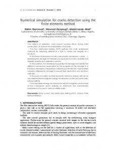
RIVER Figure 1: The simplified problem of two partially penetrating wells. Only confined flow exists in the aquifer, and it is impervious on three sides, as well as the top and bottom. The remaining side, however, is recharged by a river modeled by a constant head of 50 ft. above the top of the aquifer. The wells are modeled by the flows, Q, and 02, being distributed uniformly on the sides of the respective wells. The permeability of the soil is 0. 1 ft./min. An analytic solution to a partially penetrating well (Figure 2) has been developed by Muskaf . The equation for the potential of a well in the simplified aquifer shown in Figure 1 can be determined from the solution of a single well by the method of image [6]. The exact solution is an infinite number of image wells. However, because the radius of influence of a well is from 500 to 1,000 ft., a first or second order approximation is typically all that is required. The small problem currently being addressed requires 29 image wells on either side of the river boundary to provide zero potential at the river. Multiple wells in an aquifer are simply handled by summing the results of the individual wells.
' t.
i ! b j f -1i
t
Figure 2: A partially penetrating well.
Transactions on Ecology and the Environment vol 30, © 1999 WIT Press, www.witpress.com, ISSN 1743-3541
Computer Methods in Water Resources IV
105
Computationally, it is easy to specify a zero potential on the part of the grid modeling the river by selecting a suitable value for the datum. In our simplified problem, for instance, HD =120 ft. The heads will all be zero or negative and represent the drawdown as a results of the pumping of the wells. Usually, one can only qualitatively analyze the grids that are used by examining such things as orthogonality, aspectratio, smoothness, etc., but, in this case, since the exact solution is known, a quantitative comparison can also be made. This offers an excellent opportunity to test some of the different options in EAGLE and different mappings to see what works best for this problem. One simply computes the percentage error for each grid point for each grid point for each grid studied. This gives an excellent way of improving the grids used in modeling wells in real-world problems rather than simply using what "looks good." 3.2
Solution for a Partially Penetrating Well
First, consider the solution for a partially penetrating well in an infinite aquifer (beyond the well's radius of influence). This will indicate how to do more complex problems using wells as well as show the scientific visualization capabilities of FAST for this application. The problem solved is the second well of the simplified problem. The pertinent data are Q = 200cfm, k=0. 1 ft/min, b = 80ft,t,, = 120ft,well radius = 2ft,and radius of influence = 480 ft. A grid is constructed first by constructing an 0 type grid (21 by 21 by 25) as if doing a fully penetrating well (the entire 120 ft) for one block and then for a second block that constitutes a plug (40 ft here with a 6 by 6 by 9 grid) to account for the well being only partially penetrating. Figure 3 shows the 0 grid representing the soil and the grid for the plug. Note that an 0 type grid could have been used for the plug, but a different type was chosen. The grids in Figure 3 use equal spacing. However, it is important to use concentrated spacing toward the well and where the well bottom touches the soil. Therefore, a second grid and solution was obtained using concentrated spacing as shown in Figure 4.
Figure 3: O Grid Equal Spacing
Figure 4: Concentrated Griding
Transactions on Ecology and the Environment vol 30, © 1999 WIT Press, www.witpress.com, ISSN 1743-3541
106
Computer Methods in Water Resources IV
compared with a much smaller elliptic grid of 13,266 nodes using the utility option in EAGLE. Figure 6 shows the isolevel plot for the two well system. Figure 7 shows flow lines (particle traces) going into thefirstwell. All flow starts at the river and ends at one of the two wells. One surprising result is that the left most flow line skips the smaller well and goes for the bigger one. The large algebraic grid of 21,266 nodes created from essentially putting together two single well grids had a maximum percentage error of 5.3 percent.
Figure 5: Grid for Two-Well Case
Figure 6: Isolevel Plot
Actually, some of this error is attributed to the truncation in the number of image wells and some is due to numerical imperfections. It seemed plausible that this grid could be significantly reduced in size by applying the elliptic grid generation techniques of EAGLE to get close to the same result. Figure 8 shows a K surface for thefirstwell for the smaller elliptic grid of 13,266 nodes. This grid yielded a maximum percentage error of 5.7 percent that substantiates the hypothesis.
Figure 7: Flow Lines Plot for One Well
Figure 8: K-Level Shaded Contour
Transactions on Ecology and the Environment vol 30, © 1999 WIT Press, www.witpress.com, ISSN 1743-3541
Computer Methods in Water Resources IV
107
3.4 Real-World Example A real-world example is presented in plan view in Figure 9 consists of a part of an aquifer containing a river crossing through the region with partially penetrating wells pumping water out of the system. Line segment EF is an impervious wall such as a slurry trench found at certain construction sites. The thickness of the aquifer varies between approximately 200 to 350 ft. Table 1 contains the soil permeability data for following three distinct regions: a) Region I with the two wells which is highly anisotropic; b) Region II under the river which is a rather impervious clay; and c) Region III with the slurry trench has soil properties of a previous sand. This problem provides an excellent opportunity to test the techniques and concepts developed thus far. The area was divided into 16 blocks or subareas as shown in Figure 9. Thirteen subareas are visible with three plugs representing the partially penetrating wells. Decoupling the geometry makes it much easier to generate the grid at times. It is certainly not necessary to have so many blocks as the mapping capability of EAGLE is extensive. However, it was done this way to give the approach a through test. Once the data fries for the surf and grid modules of EAGLE were developed for a particular type of region, it was very easy to modify these fries for the next similar type region. After all the pieces were generated, it was a simple matter to combine the pieces into a single, complete FEM grid using the program developed as part of this work. Eleven layers (K levels) were used with the resulting FE grid having 11,578 nodes and 9,855 elements. With the head at the river being 300 ft, the wells each having a penetration of 1 00ft,and a head of 260 ft at the well.
Figure 9: Part of an Aquifer
Figure 10: Shaded Contour of Total Head
The grid around each well was generated by going directly from a circle to a rectangular type region with care to use gradually increasing spacing. For some applications there may be too much skewness, and an alternate plan such as a five-region system must be implemented. However, good results were achieved in this application using the original approach. The impervious wall
Transactions on Ecology and the Environment vol 30, © 1999 WIT Press, www.witpress.com, ISSN 1743-3541
108
Computer Methods in Water Resources IV
can be easily handled by having nodes at different positions on the sides of the wall. The unconfmed flow problem was run for the soil conditions in Table 1, requiring time of 3763.2 sec on the Cray YMP and five iterations for convergence. An important aspect of groundwater flow is the amount of flow from the wells. The three wells pump a total of 512.7 cfm, which is within their range of capacity. Figure 10 shows the shaded contour plot for unconfmed flow. Now, the less previous region with the two wells has more head loss that is correct. The free surface algorithms can be tested by viewing the free surface at a well. Many other plots can be obtained, but these are left to the interested users to generate. REGION 8c c Vc kp, k* kp3
I 21° -53° 10° Ix If)'" 15 x to-" 1 x 10''
II 0° 0° 0° Ix 10-' Ix 10-' Ix 10'S
III 0° 0° 0° Ix 10'' Ix 10-' Ix 10-'
Table 1 Properties of Soil Permeability (kpi in ft/min) 4. CONCLUSION The techniques and tools developed by aerospace engineers can be extremely helpful in groundwater flow problems. Also, visualization techniques are essential and a valuable tool for understanding and validating the results. An area of future research is the application of these techniques and tools to multiphase flow of groundwater with contaminant transport. REFERENCES 1.
Bancroft, Gordon, Kelaita, Paul, McCabe, Kevin, Merritt, Fergus, Plessel, Todd, Globus, AI, and Semans, John. Flow Analysis Software Toolkit (FAST). Sterling Federal System, Inc., NASA Ames Research Center, Moffett Field, CA. (1991).
2.
Muskat, M. The Flow of Homogeneous Fluids through Porous Media, Ann Arbor, MI: J. W. Edwards, Inc., pp. 263-268. (1946).
3.
Thompson, J.F. and Gatlin, B. Program EAGLE User's Manual, Volume 1: Introduction and Grid Applications. USAF Armament Laboratory Technical Report AFATL-TR-88-117, Eglin AFB, FL. (1 988a).
Transactions on Ecology and the Environment vol 30, © 1999 WIT Press, www.witpress.com, ISSN 1743-3541
Computer Methods in Water Resources IV
109
4.
Thompson, J.F. and Gatlin, B. Program EAGLE User's Manual, Volume 2: Surface Generation Code. USAF Armament Laboratory Technical Report AFATL-TR-88-117, Eglin AFB, FL. (1988b).
5.
Thompson, J.F. and Gatlin, B. Program EAGLE User's Manual, Volume 3: Surface Generation Code. USAF Armament Laboratory Technical Report AFATL-TR-88-117, Eglin AFB, FL. (1988c).
6.
Told, David K. Ground Water Hydrology, New York: Wiley & Sons, Inc., pp. 100-103.(1959).
7. Tracy, F.T. Application of Finite Element, Grid Generation, and Scientific Visualization Techniques to 2-D and 3-D Seepage and Groundwater Modeling. Ph.D. Dissertation Submitted to the Faculty of Mississippi State University. (1991).