First-break deformable-layer tomostatics constrained by shallow reflections. Hua-wei Zhou*, Hui Liu, and Fan Jiang, Texas Tech University. Peiming Li, BGP.
Main Menu
First-break deformable-layer tomostatics constrained by shallow reflections Hua-wei Zhou*, Hui Liu, and Fan Jiang, Texas Tech University Peiming Li, BGP Summary Tomostatics using first breaks is a popular way to estimate near-surface statics due to the presence of low-velocity weathering zone. However, it is difficult to constrain the geometry of the base boundary of the weathering zone using first breaks, because the corresponding raypaths tend to be parallel with this boundary, traversing on top of the basement layer. We devise here a method of first-break deformable-layer tomostatics with constrains on the depth range of the base boundary of the weathering zone using reflections. Initial test of the method is conducted using a 2D field data set from western China. Comparison between the unconstrained and constrained tomographic models shows a similar geometry of the model layers, but the constrained portion of the base boundary of the weathering zone tends to have a sharper velocity contrast and laterally smoother than that of the unconstrained model. At many places greater than 10 ms difference exists in one-way vertical traveltimes over the weathering zone of the two models, meaning large difference in their static corrections. Introduction According to Sheriff (1991), static corrections are “corrections applied to seismic data to compensate for the effects of variations in elevation, weathering thickness, weathering velocity, or reference to a datum.” A practical way to derive static corrections for onshore reflection data is first-break tomostatics which determines the near-surface velocity model using first-break tomography and then computes the time corrections for reflection traces (e.g., Docherty, 1992; Zhu et al, 1992; Al-Rufaii et al., 2001; Chang et al., 2002). In areas of complex near-surface conditions large velocity contrast often exists across the boundary between the weathering zone and basement rocks, and the thickness of the weathering zone may also possess strong lateral variations. In such cases, first-break tomostatics becomes ineffective because the thickness variation of the weathering zone cannot have much impact on the first-break traveltimes due to the fact that the deep portions of the first-break raypaths are traversing along the base boundary of the weathering zone. One possible remedy is to use shallow reflections from the base of the weathering zone to constrain the thickness of the zone. The large velocity contrast between the weathering zone and the underlain basement rocks means a strong reflection coefficient across their boundary. In such cases, the thickness of the weathering zone could be well constrained by the traveltimes of the reflections. However,
SEG Las Vegas 2008 Annual Meeting
the appearance of shallow reflections may be sporadic on the same profile, often appear in gullies with thick weathering zone and disappear near crests due to strong ground roll noise and thin weathering zone (Figure 1).
(d)
(b) (a)
(c) (a)
(b)
Shallow reflections
(c)
(d)
Figure 1: A topographic profile (top) and four shot gathers (ad) with shot locations denoted by the colored bars. Note that the shallow reflection tends to appear over gullies and masked by ground rolls over crests.
3224
Main Menu
Reflection-constrained DLT
In this study, we apply the deformable-layer tomography (DLT) method (Zhou, 2006) to the study of near-surface statics using both first breaks and shallow reflections. The shallow reflections here are referred to those reflected from or around the base of the weathering zone. Unlike the conventional tomography methods that determine the velocity values of a pre-defined grid of nodes or cells, DLT directly determine the geometry of interfaces of a set of velocity layers such as the weathering zone and basement. Considering the sporadic appearance of shallow reflections corresponding to the base boundary of the weathering zone, we pick the range or minimum and maximum traveltimes of each basal reflection and used them as a pair of constraints in the subsequent first-break tomography.
Method considerations Usage of the shallow reflections Though it is clear that using shallow reflections shall help constraining the geometry of the base boundary of the weathering zone, a key question is how to use the reflections. One difficulty is that not only the appearance of the shallow reflections is sporadic (Figure 1), but also that such shallow reflections occur only within a small offset range from each shot. Therefore, it is not a viable idea to make a simple joint inversion of first breaks and reflection traveltimes, because the reflection data is heavily outnumbered by the number of first breaks and the reflection data exist only sporadically and unevenly along the profile. Another difficulty is that the accuracy of picking reflection times is strongly influenced by the phase, bandwidth, and particularly the time duration of the reflection wavetrain, which may be regarded as a convolution of the incident wavelet with the reflectivity function across the base boundary. If the boundary is a sharp one on the impedance profile, there shall be not much difference between the incident wavelet and reflection wavetrain. However, if the boundary has a small gradient on the impedance profile, the time duration of the reflection wavetrain might be significantly widened. In such case, it is probably reasonable to use the time range, or the minimum and maximum times of the reflections. Based on the above analysis, we decide to take the traveltime ranges of all shallow reflections as constraints in the first-break tomographic inversion. The processing flow includes the following steps: 1. Picking of the first breaks and assessment of the data quality and model dimensions; 2. Unconstrained first-break deformable-layer tomography to establish the initial near-surface velocity model;
SEG Las Vegas 2008 Annual Meeting
3. Prediction of the reflection times from all possible interfaces around the base of the weathering zone using the current velocity model (from Steps 2 or 6); 4. Analysis for the validity of shallow reflections from the base of the weathering zones on shot or CMP gathers in comparison with reflection time predictions from Step 3; 5. Picking of the traveltime range of each validated shallow reflection and assigning its lateral location at the midpoint between shot and receiver positions; 6. First-break deformable-layer tomography using reflection time ranges picked from Step 5 to constrain the depth ranges of the base of the weathering zone along the profile. The above Steps 3-6 may be re-iterated several times to assure the quality of the reflection time picks. As a simplification, we may just pick a single pair of minimum and maximum reflection times at zero offset from each shot gather. Multi-scale deformable-layer tomography Both the unconstrained and constrained inversions take the DLT approach, which is motivated by two observations. Firstly, most near-surface geologic features, such as the weathering zone and stratigraphic beddings, resemble thickness-varying layers and pinch-outs rather than regularly spaced blocky cells. Secondly in nearly all cases the range of the velocity values is known a priori to velocity model building, based on surface geology, well logs, and previous seismic studies. What we want to find is the spatial position of some interesting velocity values, such as that for the weathering zone, water, sands, limestone, salt, etc. Therefore, it makes more sense if we can determine the spatial position of major velocity contours, rather than determining velocity as a function of space. The objective here is to determine the geometry of major velocity interfaces with a minimum number of model variables adapting to the geologic configuration. One important and powerful constraint for applying the DLT is the use of a priori velocity information. It is most desirable to take the velocity values or the ranges of their variation as input to the tomographic velocity model building process. The main reason is to reduce the impact of the trade-off between lateral velocity and thickness variations of the weathering zone or other layers due to the depth and velocity ambiguity (Docherty, 1992). The inversion of the DLT follows a multi-scale scheme to cope with uneven ray coverage and balance the long- and shortwavelength component of the solution model (Zhou, 2003). The basic idea is to decompose the solution updates of velocities or interfaces into components of various spatial sizes called sub-models, and to simultaneously invert for
3225
Main Menu
Reflection-constrained DLT
solutions of all sub-models. The final solution is simply a stack, or spatial superposition, of all sub-model solutions. The application of the reflection time constraints is straightforward in the iterative tomographic process. Using the current reference velocity model, each pair of minimum and maximum reflection times will be converted to minimum and maximum depths of the base boundary of the weathering zone at the corresponding lateral location. Since the velocity values of the weathering zone layers and the basement layer are approximately know prior to the inversion, the model velocity interface corresponding to the base boundary of the weathering zone will be confined within the depth ranges from the reflection data. Initial test result
0
(a) Initial reference model for DLT
Depth [m]
0 (b) Constrained DLT model
Depth [m]
(b) Constrained DLT model
467
(c) First-break rays in the final model
0 (c) Reflection depth constraints
Distance [m]
17,788
Depth [m]
Depth [m] 467 0
Depth [m]
(b) Final model after the unconstrained DLT
467 0
0 (a) Unconstrained DLT model
467
467 0
We further carried out Steps 3, 4, and 5 of the processing flow to identify shallow reflections from layers around the base boundary of the weathering zone. This process resulted in 158 pairs of reflection time ranges being picked within a distance range from 247 to 8,860 m. These reflection time ranges were used as constraints in the last step of constrained first-break deformable-layer tomography. Within each tomographic inversion iteration, each reflection time range (minimum and maximum reflection times) was converted into depth range (minimum and maximum depths) of the corresponding reflector using the current velocity model.
Depth [m]
An initial test of the new method has been conducted using a 2D field data set from northwestern China. The data are very noisy with strong ground rolls, and the shallow reflections are hardly visible (see Figure 1). The survey is split-spread with 239 shots and 480 receivers for each shot. The shot interval is 80 m and receiver interval is 40 m.
after eleven iterations of tomographic inversion. The iteration is stopped because further iterations will not produce significant reduction in data misfit level and change in the solutions. The solution shown in Figure 2b marks the completion of the Step 2 of the processing flow discussed in last section.
467
0
Distance [m]
10,000
Figure 2: (a) The initial reference velocity model. (b) The final velocity model after 11 DLT iterations. (c) First-break rays in the final model.
Figure 3: Comparison between (a) unconstrained DLT model and (b) constrained DLT model in the distance range covered by the reflection time constraints. (c) Red bars denote the depth range constraints which were converted from the reflection time range constraints using the constrained DLT model.
Figure 2 shows the initial and final velocity model of the unconstrained DLT for the field data, as well as the ray coverage of the first breaks. The final model is the solution
A comparison between the unconstrained and constrained first-break DLT models is given in Figure 3, for the
SEG Las Vegas 2008 Annual Meeting
3226
Main Menu
Reflection-constrained DLT
distance range covered by the reflection time constraints. A general similarity exists between the unconstrained and constrained models in the geometry of model interfaces. With respect to the unconstrained model, the constrained model has a sharper velocity contrast across the base boundary of the weathering zone, because the corresponding velocity interfaces within 1.8-2.7 km/s are more closing together that that in the unconstrained model. These interfaces also show a higher level of lateral smoothness in the constrained model in comparison with that in the unconstrained model. To address the impact of the velocity model on the static corrections, we computed one-way vertical traveltime throughout the weathering zone (top 400-m depth range) in the two models and plot the difference of the traveltimes in Figure 4. Notice that at some places 10-ms difference exists in one-way vertical traveltimes through the two models. Because that the static correction for each reflection trace include the one-way vertical correction for the shot location plus another one-way vertical correction for the receiver location, the potential difference in static correction between the two models can be greater than 20 ms, which is close to the period of main data frequency.
Discussion and conclusions Although tomostatics based on first breaks is a viable means to determine the near-surface velocities, the thickness of the weathering zone cannot be well constrained by first breaks when the raypaths are mostly parallel with the interface between the weathering zone and the basement, which is the most common situation when shots and receivers are placed along or near the surface. Combining the above notion with the contrasting orientations between the sub-horizontal rays of first breaks and the sub-vertical rays of reflections suggest that the static corrections of reflection times based on first-break velocity models can be problematic. In this study we experiment the use of shallow reflection times from the base of the weathering zone in the tomostatics process. The sporadic appearance of such shallow reflection makes it difficult to conduct a joint inversion of first break and reflection traveltimes. In addition, because that the reflection wavetrain from the base of the weathering zone could be significantly wider than the time duration of the incident wavelet, we decided to pick the minimum and maximum reflections times for each recognizable reflection wavetrain from the base of the weathering zone. We took such reflection time ranges to constrain the first break deformable-layer tomography in which the base boundary of the weathering will be confined within the reflection depth range at each lateral location.
ΔT [ms]
In conclusion, we have devised a method of first-break deformable-layer tomostatics with constrains on the depth range of the base boundary of the weathering zone using reflections. The initial testing of the method with a field data from western China indicates that the constrained model tends to have a sharper vertical velocity contrast across the base boundary of the weathering zone than that of the unconstrained model. The constrained model also shows a higher level of lateral smoothness than that of the unconstrained model. At many places greater than 10 ms difference exists in one-way vertical traveltimes through the weathering zone of the two models, meaning a significant difference in their static corrections. This study needs to be carried out further to make the above statement more conclusive. Distance [m]
Figure 4: Differences between the one-way vertical traveltimes in the unconstrained DLT model in Figure 2b and the constrained DLT model in Figure 3a, as a function of horizontal position in the models. Each one-way vertical traveltime is computed from the surface down to the bottom of each model.
SEG Las Vegas 2008 Annual Meeting
3227
Main Menu
EDITED REFERENCES Note: This reference list is a copy-edited version of the reference list submitted by the author. Reference lists for the 2008 SEG Technical Program Expanded Abstracts have been copy edited so that references provided with the online metadata for each paper will achieve a high degree of linking to cited sources that appear on the Web. REFERENCES Al-Rufaii, K., H. Zhou, and L. Lu, 2001, Tomographic velocity analysis in complex areas: 71st Annual International Meeting, SEG, Expanded Abstracts, 748–751. Chang, X., Y. Liu, H. Wang, F. Li, and J. Chen, 2002, 3D tomographic static correction: Geophysics, 67, 1275–1285. Docherty, P., 1992, Solving for the thickness and velocity of the weathering layer using 2D refraction tomography: Geophysics, 57, 1307–1318. Sheriff, R. E., 1991, Encyclopedic dictionary of exploration geophysics: SEG. Zhou, H., 2003, Multi-scale traveltime tomography: Geophysics, 68, 1639–1649. ———2006, Multiscale deformable-layer tomography: Geophysics, 71, R11–R19. Zhu, X., D. P. Xista, and B. G. Angstman, 1992, Tomostatics: Turning-ray tomography + static corrections: The Leading Edge, 11, 15–23.
SEG Las Vegas 2008 Annual Meeting
3228