First-Order Probabilistic Models for Predicting the Winners of Professional Basketball Games David Orendorff
[email protected]
Todd Johnson
[email protected]
December 12, 2007
1
Introduction
2
Background
Probabilistic methods for learning and inference are by no means a recent phenomenon. However, the popularity of these techniques in artificial intelligence, machine learning, and related areas (such as bioinformatics and computational biology) has grown dramatically since the development of compact graphical representations, and in particular Bayesian networks and Markov random fields [5]. These frameworks have facilitated the development of general algorithms for learning and inference, which could then be leveraged by any model, in any domain. Even as these tools have grown in popularity, they have also shown their weaknesses. One of the most important of these is an inability to capture abstract or high level structure exhibited by many real-world datasets. For instance, a researcher who wishes to model a database containing the medical records for cancer patients using a Bayesian network must specify explicitly a node for every attribute of every patient, and the links between these. In this way, the expressive power of Bayesian networks and Markov random fields is not unlike that of propositional logic. Propositional logic has the power to prove any statement which does not contain quanti-
There have been several recent attempts to extend propositional probabilistic frameworks such as Bayesian networks and Markov random fields to handle higher-order relationships, analogous to the way in which first order logic extends propositional logic. Perhaps the two most well known are Bayesian Logic (BLOG) and Markov Logic Networks (MLNs). To date there have been very few (if any) unbiased comparisons of these packages applied to large problems. We begin to address this issue by formulating the same prediction task as a model in each of these languages, in order to gain insight into each framework’s strengths and weaknesses. In particular, this project considers the task of predicting the winner of professional basketball games based on historical data. Prediction accuracy of models implemented in the BLOG and MLN frameworks are compared using cross validation for the 2006-2007 season. We conclude with a discussion of the experience of solving a non-trivial problem in each language. 1
2.2
fiers, but every fact about the world, every relationship between two or more entities, must be expressed with its own atom. It is then natural to consider ways of extending probabilistic graphical models to handle higher-order relationships, in the way that first-order logic extends propositional logic to encompass relations and quantifiers. That is, we would like to allow our hypothetical cancer researcher to express once the relationship between a person’s white blood cell count and his chances of having cancer, and to have our model understand that this relationship holds for every test conducted on every person in their database. Many attempts have been made along these lines, including [1], [2], [3], [4], and [6]. While an in-depth discussion of the either framework is beyond the scope of this paper, we briefly review Markov logic networks and Bayesian logic, the two most fully-formed firstorder probabilistic languages.
2.1
Bayesian Logic
Bayesian logic (BLOG) provides a way of succinctly specifying a generative model. Syntactically, these models resemble programs in a typed first-order logic programming language, such as λ-Prolog: they consist of predicates, clauses, and dependency statements. Semantically, however, a BLOG model represents a type of (potentially infinite) Bayesian network called a contingent Bayesian network. Each possible grounding of each predicate is given a node in the network, and the nodes are connected to the propositions on whom they logically depend in the model.
2.3
Predicting the Outcome of Sports Events
Professional sports have been the focus of a great deal of statistical inquiry. Numerical hobbyists and professional statisticians alike have poured hours into analyzing batting averages, devising statistical measures for rating player performance, and predicting the outcomes of games. The statistical journal Chance, published by the American Statistical Association, formerly ran a regular column entitled “A statistician reads the sports page,” written by UC Irvine professor Hal Stern. The reasons for this interest are many, but include the fact that professional sports simply provide a wealth of data for statisticians. Predicting the outcomes of individual games in professional sports is a particularly interesting task. One reason for this is that we understand that the outcomes are governed by unknown factors, such as the skill levels of the individuals and teams involved. Therefore, we hope the raw data may hide some underlying structure, which can be leveraged to make more accurate predictions. Another reason is that there is money to
Markov Logic Networks
Recall that an MLN can be thought of as a set of first order clauses with weights. The inference task is to estimate the probability of each grounding of some non-evidence predicates. Likewise, the MPE task is to determine the most probable explanation given the data and the network. Alchemy is an implementation of MLN inference, weight learning and structure learning. It can be found at http://alchemy.cs.washington.edu/. For inference and weight learning Alchemy takes in a .mln file and a database file (evidence). Inference is typically fast (around a few minutes). Likewise, structure learning takes as input an mln file (optional) and database file. 2
Sport Pro football Pro basketball Pro baseball College football College basketball
Home Team .58 .66 .53 .62 .68
Win/Loss .63 .69 .56 .69 .72
Scores .65 .70 .56 .73 .72
Oddsmakers .67 .71 .55 .75 .75
Table 1: Probability of correctly guessing the outcome of a game given a prediction method. Taken from [7].
be made by predicting the outcomes of sporting events. Professional oddsmakers predict the outcome of every game, and survive on their ability to do so with higher accuracy than the public Figure 1 shows the percentage of correct predictions by three simple predictors, and by professional oddsmakers, who we take to be domain experts. The first predictor always predicts that the “home team” will win. The second always predicts that the team who has won more games before the query game will win. The oddsmakers presumably take into account domain knowledge such as strengths and weaknesses of each team, which players are injured on a given day, as well as which team is at home and how each team has performed so far this year. This data represents the state of the oddsmaking art, as of 1997 [7]. The predictions in this work are based on the 2006-2007 season of the National Basketball Association (NBA). The NBA has thirty teams, divided into two fifteen-team conferences. During the season, each team plays against every team in the other conference twice, and against every team in its own conference either three or four times. We consider a database of observations of the form (teamA, teamB, k, w), where each entry represents the results of one game, such that teamA and teamB are teams, this entry corresponds to the kth time the teams have
played against one-another this season, and w ∈ {teamA, teamB} is the winning team. There are 1230 games during the course of the season; for each trial, we will observe 1130 games and attempt to predict the outcome of the remaining 100. In order to generate predictions, we will query our models for the marginal probability distribution which governs the outcome of each held-out game, and we will predict that the team which the model assigns a higher posterior probability of winning will in fact do so.
3
MLN Model
As models evolved it became apparent (although in hindsight it should have been obvious) that models with more clauses to ground in the network generally resulted in worse performance. As an example, we wanted a transitive property– saying that A beats B and B beats C implies A beats C. However, since there is an (implied) universal quantifier in front of each clause, the clause requires O(n3 ) groundings for each unique tuple of (A, B, C). If we also have game ids for each of the predicates in the transitive clauses, while correct logically, the space required for inference grows by a factor of 10-100. Indeed, our first models exhibited this behavior and only af3
ter further analysis did we migrate towards a model with hidden nodes. To date, the best performing model has a hidden BetterT han(teamA, teamB) predicate and an observable W inner(teamA, teamB, game id)) predicate. The actual code is in Figure 1. The first rule ending in ‘.’ is a hard constraint stating that if a teams is better than another, the other is worse than this team. The next clause indicates how the outcome of a particular game affects the BetterThan predicate. The third clause is the transitive property, saying that t1 > t2 and t2 > t3 =⇒ t1 > t3. The weights were learned with two different methods and then the performance was compared. Discriminate training took around 3 minutes. Generative learning took about 2 seconds. The accuracy of the two using leave 100 out validation was within 2 percent of each-other. So it is not clear which method works better.
4
game. Specifically, the probability of each team winning a given game is a function of the difference between their relative qualities. In particular, if we let q = Quality(teamA) − Quality(teamB), then the probability that teamA will win is given by 1 q , where θ is a hyperparameter set to 10 1+e θ
throughout these experiments. This relationship makes up the last four lines of the code for the model. The rest of the code sets up the known objects in each possible world, and gives us a way to generate games played between teams. In addition to the BLOG code given here, the model consists of approximately 600 lines of Java code, dispersed over six classes. Five of these classes implement functions named in the BLOG model: BasketDiffConfCPD and BasketSameConfCPD, which represent the probability distributions for the number of games played by two teams, given that they are in the same or different conferences, respectively, ConfAssignment, and TeamOrdering, which implement nonrandom bookkeeping functions, and BasketSigmoidCPD, which implements the sigmoidal conditional probability distribution discussed above. A sixth class, BasketGibbsProposer, which contains the bulk of the Java code, implements a custom proposal distribution for the MetropolisHastings algorithm. This proposal distribution approximates Gibbs sampling by attempting to sample each variable from a distribution which is as close as possible to the distribution given by observing the variable’s Markov blanket, while still being computable in a reasonable amount of time. Since the Poisson prior and the sigmoidal conditional propabilities are not conjugate, we were unable to derive a closed form for the
BLOG Model
The BLOG model developed for this problem is given in Figure 2. The intuition behind the BLOG model is that it encodes a Bayesian network described as follows. First, there is a variable for each game, which is an observable, or leaf, node. Then there is, associated with each team, a hidden variable, which represents the quality of that team. This may be thought of as some measure of the team’s talent, or its skill, or its desire to win, or its luck, or whatever singular property most distinguishes a good team from a bad one. When two teams play, their relative qualities determine which team is most likely to win, so each game node has as parents the quality nodes of the two teams participating in that 4
// predicates Winner(team, team, game) BetterThan(team, team) // rules BetterThan(t1,t2) !BetterThan(t2,t1). w1 Winner(t,t’,g) => BetterThan(t,t’) w2 (BetterThan(t1,t2) ^ BetterThan(t2,t3)) => BetterThan(t1,t3) Figure 1: MLN Model
5
probability of a team’s quality given the rest of the network. Therefore, when we wish to sample a quality node, we approximate the conditional distribution by computing the total joint probability of the node and its Markov blanket for each of 21 possible values. We then normalize these 21 probabilities so that they sum to one, and sample a new value from this distribution. In general, these 21 values contain by far the bulk of the probability density, but the algorithm is nonetheless only an approximation to Gibbs sampling.
Results
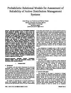
Here we compare the prediction accuracy of the MLN model, the BLOG model, and a simple baseline predictor. The baseline predictor just counts the total number of wins by each team, and for a given game always predicts that the team which has the higher win total will win again. Figures 3 and 4 summarize our results. Figure 3 displays a histogram for each predictive method, with predictive accuracy on the x-axis and number of trials in which this accuracy was achieved along the y. The same information is summarized in Figure 4, which shows the mean and standard deviation of the prediction accuracy for each method, across 100 trials of leave100-out testing. The MLN model performs far better than either of the other two models, displaying a higher average accuracy (76%) and lower variance. The BLOG model performs almost identically to the baseline predictor, with 64% accuracy for the baseline and 63% accuracy for the BLOG model, and a 4% standard deviation in each case. This makes sense in the following light: each of these predictors bases its guess for each game on a single quantity related to each team (total wins
This proposer achieves nearly 100% acceptance of proposed moves, and improves over the speed of the provided generic MetropolisHastings sampler enormously. The provided proposer takes an hour to generate 500 samples, none of which are accepted. This means that hours are spent performing ‘inference,’ but nothing is happening; at the end, all you find out is that the model was unable to generate any acceptable proposed states. Our proposer generates 500 samples in 45 seconds, and in general greater than 95% are accepted. 5
type Team; type Conference; type Game; random NaturalNum Quality(Team); random Team Winner(Game); nonrandom Conference Conference(Team) = blog.ConfAssignment; nonrandom NaturalNum TeamId(Team) = blog.TeamOrdering; guaranteed Conference East, West; guaranteed Team BOS, NYK, TOR, NJN, PHI, CHR, ORL, WAS, MIA, ATL, IND, CHI, DET, CLE, MIL, SAS, DAL, MEM, HOU, NOO, PHO, LAL, LAC, GSW, SAC, POR, SEA, MIN, UTA, DEN; generating Team FirstTeam(Game); generating Team SecondTeam(Game); #Game(FirstTeam = teama, SecondTeam = teamb) { if TeamId(teama) < TeamId(teamb) & Conference(teama) != Conference(teamb) then ~ BasketDiffConfCPD() elseif TeamId(teama) < TeamId(teamb) then ~ BasketSameConfCPD() }; Quality(t) ~ Poisson[15]; Winner(g) ~ BasketSigmoidCPD(FirstTeam(g), SecondTeam(g), Quality(FirstTeam(g)), Quality(SecondTeam(g))); Figure 2: BLOG Model
6
0.8
Baseline (most wins) 20
0.75
10 0 0.5
0.55
0.6
0.65 pct correct
0.7
0.75
Average Percent Correct
density
30
0.8
MLN with hidden variables density
30 20 10 0 0.5
0.55
0.6
0.65 pct correct
0.7
0.75
0.7
0.65
0.8 0.6
BLOG density
10
5
0.55
0 0.5
0.55
0.6
0.65 pct correct
0.7
0.75
MLN
BLOG
0.8
Figure 4: Means and standard deviations of prediction accuracies.
Figure 3: Percentage of correct predictions, using a leave-100-out scheme.
the 2006-2007 season. While the two numbers are within one standard deviation of the predictive power of the baseline model in our experiments, the size of the difference is interesting. One difference, which we assume exists between our baseline and this predictor, is that our baseline model does not take time into account, so it does not restrict its attention only to wins before the game to be predicted, but counts all of a team’s wins in the training set. This makes the baseline a more reasonable comparison for our methods, which also do not take time into account. However, it seems as though this should only improve the power of the predictor, so it does not explain the noted discrepancy. We also note that the MLN model does somewhat better than the reported accuracy of the oddsmakers in [7]. However, the same caveat as above applies here: our model has access to both past and future games from within the same season when predicting winners. Further, we must assume that advances have been made in the state of the oddsmaking art since 1997. Fi-
for the baseline, quality for the BLOG model). We had hoped that there might be some fine distinction between these two quantities, which the BLOG model might be able to tease out, thereby improving performance. For instance, the BLOG model can penalize a team’s quality less when it loses to a good team than when it loses to a bad team, while total wins is oblivious to this distinction. However, it seems as though, to the extent that these nuances exist in the data, they are washed out over the course of an NBA season, and the two predictors are simply comparable.
6
Baseline
Discussion
We note that Table 1 indicates a 69% accuracy when guessing the team with the most previous wins as the winner of a game, which is a bit higher than the 64% accuracy displayed by the baseline measurement in our experiments for 7
ative qualities. Markov logic does not, as far as we could discover, have a way to specify the weight of the clause which encodes “teamA beats teamB” as a deterministic function of attributes of the two teams. Markov logic does have the ability to learn, based on some data, a different weight for each possible grounding of a clause. The extent to which this would be a way to implement the same model in a MLN, and the exA Note on Comparing the Two tact relationship of this learning to inference on the same dataset, remains unexplored. Models
nally, no variance or error measure was given for the accuracy of the experts. Therefore, we cannot conclusively say that our models do better than a human expert. Nonetheless, given that even in 1997 the experts had access to enormous amounts of domain knowledge, the 3.5% difference between our MLN model and the oddsmakers is encouraging.
6.1
One stated goal of this work is to compare MLN and BLOG models. It is tempting, then, to look at Figure 4 and conclude that Markov logic networks carried the day. While there is some sense in which this is true, we should not be quite so hasty. To begin with, let us reinforce something which should be obvious: we implemented two completely different models, one in each language. In the simplest terms, the model built in Markov logic has N 2 hidden variables, compared to only N for that built in BLOG. If it did not perform better, we should be very surprised. So, to the extent that the MLN model outperforms the BLOG model, this is entirely because it is a better model for the task at hand, and, a priori, has nothing to do with the two languages. However, neither of these models arose spontaneously, and it is in the process of creating a model where MLNs take the lead. The first model we designed was the model implemented in BLOG. It is a very intuitive model, which seems to be true of most BLOG models. Writing the BLOG model in Figure 2 was nearly trivial, while coding the same model in Markov logic turns out to be more complicated. The blog model assigns a variable probability to teamA beating teamB, based on their rel-
Instead, one author set about finding another model in Markov logic, while the other began writing a custom Metropolis-Hastings proposer for the BLOG model. This turned out to be a time consuming and non-trivial task, and required the author to become intimately acquainted with the Java code which runs BLOG. After about a week of work, we had a proposal distribution in Java, specific to the model in Figure 2. Once this was complete, it became clear that the model would not be able to outperform the baseline. At this point, the process of writing a new model, then writing a new proposer, and finally running more tests, would have taken us far beyond the deadline for this project. Meanwhile, the other author was able in the same time to try many different MLN models, each of which required a trivial amount of time to both code and evaluate. In this way, we were able to hit upon a good model by a process of trial, experimentation, error, and revision. This, then, is the true sense in which MLNs can be said to have won the comparisson: by allowing fast evaluation and revision of a model, the MLN framework allowed much greater freedom to explore the space of possible models. 8
6.2
Lessons Learned: MLNs
for observed games; adding hidden variables to encode a team’s offensive and defensive abilities separately; and explicitly modeling time as the season progresses. Finally, we would also like to consider more sophisticated ways of using the marginal posterior probability of each team winning than simply choosing the most likely winner. It would be interesting to investigate error metrics which leverage the uncertainty of a 51/49 split in the posterior probability, versus the near-certainty of a 95/5 split, as posterior probabilities of all of these types were routinely observed.
Working with MLNs allows us to suggest rules of thumb that may be useful for future MLN endeavors. For example, it is vital to use the correct open world or closed world assumption. The wrong decision can strongly reduce accuracy and increase search space size. Furthermore, it is generally a good idea to have a rule for each unit literal. This way the model has a prior distribution to start from. This is especially useful when using implication rules. Since implications are true whenever the ‘cause’ is false and the antecedent may be true with artificially high weight.
6.3
References
Lessons Learned: BLOG
[1] Nir Friedman, Lise Getoor, Daphne Koller, and Avi Pfeffer. Learning probabilistic relaAs noted above, the BLOG model implemented tional models. In Proceedings of the Internafor this problem is very simple, as it considers tional Joint Conferences on Artificial Intellionly a binary variable for the outcome of each gence, pages 1300–1309, 1999. game and a single integer-valued variable for the performance of each team. This simplicity was [2] David Heckerman, Christopher Meek, and Daphne Koller. Probabilistic entitya design decision at the outset, as preliminary relationship models, prms, and plate models. attempts to model simple problems, such as a In Proceedings of the ICML-2004 Workshop probabilistic mixture model for clustering, met on Statistical Relational Learning and its with essentially terrible results. However, it is Connections to Other Fields, Banff, Canada, now clear that most of these problems were due 2004. to the inefficient generic sampling schemes provided with BLOG. [3] Brian Milch, Bhaskara Marthi, and Stuart It seems probable that, given an intelligent Russell. Blog: Relational modeling with custom proposal distribution and enough time, unknown objects. In Proceedings of the BLOG should be able to handle inference on a ICML-2004 Workshop on Statistical Relareasonably complex model. Therefore, if we had tional Learning and its Connections to Other anything to do over, it would be to enrich the Fields, Banff, Canada, 2004. BLOG model. Ideas that we have had include an encoding for which team is the “home team,” [4] Eric Mjolsness. Variable-structure systems and possibly shifting the sigmoidal conditional from graphs and grammars. Technical Reprobability to favor the home team; representport ICS 05-09, University of California, ing not only the winning team, but final scores Irvine, October 2005. 9
[5] Judea Pearl. Probabilistic reasoning in intelligent systems: networks of plausible inference. Morgan Kaufmann Publishers Inc., San Francisco, CA, USA, 1988. [6] Matthew Richardson and Pedro Domingos. Markov logic networks. Machine Learning, 62(1-2):107–136, 2006. [7] Hal S. Stern. How accurately can sports outcomes be predicted? Chance, 10(4):19–23, 1997.
10