First Order Quantum Phase Transition in Adiabatic Quantum

First Order Quantum Phase Transition in Adiabatic Quantum Computation M. H. S. Amin1 and V. Choi1, 2

arXiv:0904.1387v3 [quant-ph] 15 Dec 2009

1

D-Wave Systems Inc., 100-4401 Still Creek Drive, Burnaby, B.C., V5C 6G9, Canada 2 Department of Computer Science, Virginia Tech, Falls Church, VA 22043, USA

We investigate the connection between local minima in the problem Hamiltonian and first order quantum phase transitions during an adiabatic quantum computation. We demonstrate how some properties of the local minima can lead to an extremely small gap that is exponentially sensitive to the Hamiltonian parameters. Using perturbation expansion, we derive an analytical formula that can not only predict the behavior of the gap, but also provide insight on how to controllably vary the gap size by changing the parameters. We show agreement with numerical calculations for a weighted maximum independent set problem instance.

I.

INTRODUCTION

Adiabatic quantum computation (AQC) was first proposed in 2000 by Farhi et al. [1] as a means to solve NPhard optimization problems. Later, Aharonov et al. [2] proved that AQC is polynomially equivalent to conventional (gate model) quantum computation. It is also believed that AQC is more robust against errors caused by environmental noise [3, 4, 5]. In AQC, the system’s Hamiltonian, usually written as H(t) = [1 − λ(t)]HB + λ(t)HP ,

(1)

evolves slowly with time t as λ(t) changes monotonically from 0 to 1 within a time tf . The initial Hamiltonian HB is assumed to have an easily accessible ground state into which the system is initialized, while the ground state of the final Hamiltonian HP provides the solution to the problem of interest. In order to reach the final ground state with high fidelity, the adiabatic theorem requires −δ tf ∝ gmin , where gmin is the minimum gap between the two lowest energy instantaneous eigenstates of H. The power δ can be 1, 2, or possibly some other number depending on the functional form of λ(t) and the distribution of the higher energy levels [1, 6, 7]. Thus, in order to address the efficiency of AQC, one needs to analyze gmin , which is unfortunately as hard as solving the original problem if computed directly. The most fundamental problem in AQC is therefore how to bound gmin analytically. Equally important is how to unveil the quantum evolution blackbox by relating the the formation of gmin to the structure of the problem, and thus obtain insights for designing efficient algorithms. Besides a few special cases in which spectral gaps are computed analytically [8], all other known studies have to resort to numerical calculations, e.g., diagonalization [9] or quantum Monte Carlo (QMC) techniques [10]. Unfortunately, these methods are limited to small problem sizes (to date, N λc , but with a much smaller number of computational states involved. As λ is increased, the total energy of such localized state will change and at some later point (λ∗ ) it may cross another localized state. The ground state of the system will then make a sudden transition to the new state via a discontinuous (first order) QPT [24]. The gap at the transition point will be extremely small, making λ∗ the new position of the minimum gap. The transition at λ∗ is between two ordered phases, in contrast to the order-disorder transition at λc . There may even be more than one such transition if the ground state crosses other localized states, but all those transitions can only happen after localization at λc . An important question now is what properties of HP are responsible for such a first order QPT. In the next section, we will employ perturbation expansion to answer this question.

III.

PERTURBATION EXPANSION

Let us define H0 = λHP and H′ = (1−λ)HB as the unperturbed and perturbation Hamiltonians, respectively. We use ζ as defined in (3) as the dimensionless small parameter. At ζ= 0 (λ=1), the eigenstates of the system are eigenfunctions of HP (computational states). Thus |ψ0 i is the global minimum of HP and the lowest lying excited states are either states that are a few bit flips away from (or neighborhood of) the global minimum, or some low energy local minima and their corresponding neighborhoods. These two types of states behave completely differently as ζ is increased. Since H′ only involves σix operators, to every order of perturbation it flips only one qubit. Therefore, the lowest order of perturbation that gives a nonzero off-diagonal element Hmn ≡ hm|H|ni is equal to the number of bit flips fmn (Hamming distance) between states |mi and |ni. This gives Hmn = O(ζ fmn ), hence at λ≈ 1 the only non-vanishing Hmn are those between neighboring states for which fnm is small. Essentially, H becomes block diagonal with every minimum

E EL(0)

0

EG(0)

gmin E*

ELP EGP 0

*

1

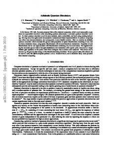
FIG. 1: Schematic diagram of crossing global and local minima. At zeroth order perturbation, levels do not cross (solid lines). Contribution from the second order perturbation may cause the levels cross if the curvature of the upper level is larger than the lower one (dashed lines).

and its neighborhood forming a cluster of states with nonzero off-diagonal elements with each other, but vanishingly small off-diagonal elements with states in other clusters. Upon diagonalization of H, the new eigenstates become superpositions of only the neighboring states. Those neighboring states never cross due to the no-levelcrossing theorem [19]. On the other hand, if as λ is decreased, two clusters move as a whole with respect to each other, as their energy levels cross they create anticrossings with very small gaps of O(ζ fmn ). The lowest of these anticrossings form a first order QPT. Let us now make the above observation more quantitative. At λ= 1 the Hamiltonian H= HP has a global minP imum |G(0) i with energy EG . Let |L(0) i represent a low energy local minimum (not necessarily the first excited state) of HP with energy ELP . For now we take both the above states to be non-degenerate. We use perturbation expansion to calculate the perturbed states |α= G, Li, and their eigenvalues Eα at λ < ∼ 1. To the second order perturbation, Eα = λEαP − χα (1−λ)2 /λ, where χα =

X |hα(0) |HB |n(0) i|2 λ3 d2 Eα . = EnP − EαP 4 dλ2

(4)

n6=α

The perturbation expansion holds as long as for all states contributing to the sum, EnP −EαP ≫ (1−λ)∆/λ. The two perturbed levels cross at (see Fig. 1)  −1 s P P EL − EG  λ∗ = 1 + , (5) χL − χG

P Since ELP >EG , if χL