1
Fixed-Interval Kalman Smoothing Algorithms in singular state-space systems Boujemaa Ait-El-Fquih and Franc¸ois Desbouvries∗
GET / INT / d´ept. CITI and CNRS UMR 5157 9 rue Charles Fourier, 91011 Evry, France ∗
corresponding author
tel +33 1 60 76 45 27, fax +33 1 60 76 44 33,
[email protected]
Abstract Fixed-interval Bayesian smoothing in state-space systems has been addressed for a long time. However, as far as the measurement noise is concerned, only two cases have been addressed so far : the regular case, i.e. with positive definite covariance matrix; and the perfect measurement case, i.e. with zero measurement noise. In this paper we address the smoothing problem in the intermediate case where the measurement noise covariance is positive semi definite with arbitrary rank. We exploit the singularity of the model in order to transform the original state-space system into a pairwise Markov model with reduced state dimension. Finally, the a posteriori Markovianity of the reduced state enables us to propose a family of fixed-interval smoothing algorithms.
I. I NTRODUCTION Let us consider the state space system xn+1 = Fn xn + Gn un yn
= Hn xn + Jn wn | {z }
,
(1)
vn
DRAFT
2
in which xn ∈ IRnx is the state, yn ∈ IRny the observation, un ∈ IRnu the process noise and vn ∈ IRnv the measurement noise. Processes u = {un }n∈IN and w = {wn }n∈IN are zero-mean, independent1 , jointly independent and independent of x0 . So xn is a Markov chain (MC) and (xn , yn ) is a hidden Markov chain with independent noise (HMC-IN). Fixed-interval smoothing consists in estimating xn from y0:N for 0 ≤ n ≤ N . In the case where the covariance matrices Qn of Gn un and Rn of vn = Jn wn are positive definite (> 0), many algorithms have been derived by using such different methods as calculus of variations [1], maximum a posteriori [2] [3], orthogonal projections [4], the innovations approach [5], the two-filter form [6] [7], complementary models [8] or the Bayesian approach [9] [10] (modern surveys can also be found e.g. in [11, ch. 10] [8] or [12]). The case where Rn is the null matrix (Rn = 0) has received less attention so far, even though it is of interest in many applications, in particular if the measurement additive noise is colored. Let us briefly summarize the existing contributions. At least two cases can lead to this situation. •
Unnoisy measurement case (wn = 0). The unnoisy measurement case was first addressed by Kalman in his original paper [13], see also [14]. A continuous time BF smoother has also been derived in [15].
•
Autoregressive (AR) measurement noise. Let wn = An−1 wn−1 + ξn
(2)
(with w0 = ξ0 ), in which ξn is zero-mean, and x0 , {un }n≥0 and {ξn }n≥0 are independent. Let x∗n be the augmented state x∗n = [xTn , wnT ]T . Then system (1) can be rewritten as the unnoisy measurement system :
x∗n+1 =
y n
Fn
0
0
An
x∗n +
Gn un ξn+1
.
(3)
= [Hn Jn ] × x∗n
The AR measurement noise case has been addressed in many papers, but up to our best knowledge, three algorithms only have been derived : the Kalman filter (KF) [16] [17] [18] [19] [20] [21], the Rauch-Tung-Streibel (RTS) algorithm [18] [20], and a fixed-lag smoothing (FLS) algorithm [21]. Remark 1: In some particular cases one can avoid increasing the dimension of the state. Let us assume that Jn is the ny × ny identity matrix Iny and that E(ξn ξnT ) > 0. Then model (1) can be 1
The independence assumptions in this paper come from our choice to adopt the Bayesian point of view and next derive our
smoothing algorithms by injecting the Gaussian assumption. Alternately, we could of course have assumed that the independent processes are uncorrelated only, and derive our algorithms as recursive linear minimum mean square error restoration procedures. DRAFT
3
x = F n n−1 xn−1 + Gn−1 un−1 y e n xn−1 + v en = H en
transformed into
(4)
e n = Hn Fn−1 − An−1 Hn−1 , and v en = yn − An−1 yn−1 , H en = Hn Gn−1 un−1 + ξn . in which y enT ) > 0, (4) is a regular state-space system, with the same Since {e vn }n≥0 is independent and E(e vn v
state xn (rather than an augmented one x∗n ), correlated process and measurement noises, and with en . For model (4) the KF has been derived e.g. in [16] [19] [20] [18], the RTS pseudo-measure y
algorithm in [20] [18], an FLS algorithm in [22] [23], and a two-filter smoother (for the continuous time case) in [24]. Remark 2: In the above models x0 , {un }n≥0 and {ξn }n≥0 were assumed to be independent, which implies that {un }n≥0 and {wn }n≥0 are independent too. Let us now only assume that x0 and {(un , ξn+1 )}n≥0 are independent, but that the subvectors un and ξn+1 are correlated. These assumptions, in turn, imply that un and wn+p are correlated for all p > 0, which can be of interest in some cases like in aircraft radar guidance systems [25], in which the system and measurement noises come from the same source, and so are correlated. Yet in (3) x∗n remains an MC, and (4) is still an HMC-IN, which implies that the algorithms for models (3) and (4) can still be used. Let us finally consider the general singular case in which Rn is a positive semi-definite matrix (Rn ≥ 0). Up to our best knowledge, only filtering has been addressed in this case [16]. Apart from the case
where Jn is not a full rank matrix, the singular measurements case also occurs when some of the measurements are either unnoisy or colored : •
n
Partially unnoisy measurements case. Let yn = [yn1 · · · yn y ]T . If some components {ynk }k∈K are unnoisy then Rn ≥ 0.
•
Partially AR measurement noise. Let some of the components be colored. Without loss of generality we thus assume that
Jn wn = [J1n J2n ]
wn1 wn2
,
wn1 wn2
=
A1n−1 0 0
0
1 wn−1 2 wn−1
+
ξn1
ξn2 | {z }
(5)
ξn
in which, again, x0 , {un }n≥0 and {ξn }n≥0 are independent. Then the AR noise block component can be concatenated to xn in order to form an augmented state x∗n = [xTn , wn1 ]T , and system (1) can
DRAFT
4
be rewritten as :
F 0 G u n n n x∗ x∗n + n+1 = 1 1 0 An ξn+1 y = [H J1 ] × x∗ + J2 ξ 2 n
n
n
n
(6)
n n
which again is an HMC-IN with singular measurement noise. Remark 3: Remarks 1 and 2 still hold, and in particular (6) remains an HMC-IN with singular measurement noise if we only assume that x0 and {(un , ξn+1 )}n≥0 are independent. In this paper we study the fixed-interval smoothing problem in model (1), in the case where Rn is an arbitrary (and possibly null) ≥ 0 matrix. We exploit the singularity of Rn in order to transform the original state-space system into an (equivalent) stochastic dynamical system but with state dimension reduced by the nullity of Rn . The transformed system happens to be a Pairwise Markov Chain (PMC) model, and as such the hidden process (even though it is not Markovian) is Markovian conditionnally on the observations. This key computational property finally enables us to develop fixed interval smoothing algorithms in the transformed system - and therefore, equivalently, in the original singular system. The paper is organised as follows. Section II is devoted to the transformation of the HMC-IN model (1) into a reduced state PMC model. In section III we propose Bayesian fixed-interval smoothing algorithms in a general (i.e., not necessarily linear and Gaussian) PMC model. Following the Bayesian point of view for deriving minimum mean-square error (MMSE) algorithms for state-space systems (see e.g. [26]), in section IV we inject the Gaussian assumption into the algorithms of section III, which eventually yields our fixed interval smoothing algorithms for singular measurement noise state-space systems. In section V we perform some simulations, and finally ection VI concludes the paper. II. S TATE - SPACE TRANSFORM We address the fixed-interval smoothing problem in the singular measurements case, i.e. in system (1) in the case where Rn ≥ 0. Some of the classical fixed-interval smoothing algorithms (see e.g. [27] for a recent review), originally designed for regular state-space systems, still hold in the singular case, but some others cannot be used any longer. In this paper we thus develop an alternative technique. Let r = rank(Rn ) ∈ {0, 1, ... , ny − 1}. Following [16], we transform the state space model (1) in order to reduce by m = ny − r the order of state xn . In sections III and IV it will remain to design smoothing algorithms for this reduced-order linear stochastic system.
DRAFT
5
A. State-space transform Since Rn has m zero eigenvalues, there exists a square non-singular matrix Mn satisfying 0 0 m , Mn Rn MTn = 0 Ir in which 0m denotes the m × m null matrix. p y n = yrn | {z } yn
(7)
Let yn = Mn yn and vn = Mn vn ; then from (1) we get p H 0 n xn + m×1 , (8) r Hn vrn | {z } | {z } vn
Hn =Mn Hn
and we see that yn is divided into a perfect part
(ypn )m×1
(the unnoisy part) and a regular one (yrn )r×1 .
Since m linear functionals of the state xn are known once yn is known, there is no need to estimate them, and this is why one can reduce by m the order of the state-space system, as we now see. Let us assume that nx ≥ m,
(9)
and that in (8) p
rank(Hn )m×nx = m. Then one can choose a (nx − m) × nx matrix Un in such a way that the transform xn (Un )(nx −m)×nx xn = p ypn (Hn )m×nx | {z }
(10)
(11)
Tn
is reversible, and finally Tn and Mn enable us to transform the original linear state-space model (1) into the equivalent state-space system x x n+1 = Tn+1 Fn T−1 n +Tn+1 Gn un . n p yn+1 ypn | {z } | {z } Tn+1 xn+1
(12)
Tn xn
On the other hand from (8) and the first equation of (1) we have
r
yrn+1 = Hn+1 xn+1 + vrn+1 x n r + Hrn+1 Gn un + vrn+1 . = Hn+1 Fn T−1 n ypn
(13)
DRAFT
6
Gathering (12) and (13), we eventually get the reduced-order linear dynamic stochastic system : x,x x,y xn+1 Fn Fn xn Un+1 0 Gn un = + , y,x y,y yn+1 Fn Fn yn Hn+1 eIr vrn+1 | {z } | {z } | {z } zn+1
with
Fn
(14)
wn
Fn = |
Tn+1 r Hn+1
{z
[Fn T−1 , 0], n | {z } } nx ×(nx +r)
(15)
(nx +r)×nx
eIr =
0m×r
.
(16)
Ir
Note that if r = 0 then equations (13)-(16) are useless, and (14) reduces to (12). Now, (12) also coincides with (14) with yn = ypn = yn (since we can take Mn = Iny ), F n = Tn+1 Fn T−1 n , and w n = Tn+1 Gn un . As a consequence the algorithms of sections III and IV, designed for model (14), also hold (up to these adjustments) in the case r = 0. B. Markovianity of the reduced state model (14) The noise of (14), {wn }n , is zero mean and independent since u and {vrn }n are independent and jointly independent. Moreover, from (15) and (11) we get T1 F 0 z0 = r F0 x0 . H1 Then w is independent of F 0 z0 (because w is independent of x0 ). For these reasons, the process {zn }n is a Markov chain (MC), so model (14) defines a so-called PMC. PMC models have been first introduced in the discrete state case and have been applied in the context of image segmentation [28]. KF for continuous state PMC has also been addressed, see [29] [30], and parameter estimation via the EM algorithm is available too [31]. The term ”pairwise” here emphasizes the fact that even though zn = (xn , yn ) is an MC, the marginal process x in model (14) is indeed not Markovian. However, in a PMC the conditional distribution p(x|y) is Markovian; this property enables the developpement of efficient Bayesian restoration algorithms, and in particular, in the context of this paper, of fixed interval smoothing algorithms.
DRAFT
7
III. BAYESIAN FIXED - INTERVAL SMOOTHING ALGORITHMS IN PMC For notational simplicity let us set xn = xn , yn = yn and zn = [xTn , ynT ]T . Let us start by the general case, i.e. the case of the non-linear and/or non Gaussian PMC model : zn+1 = g(zn , wn ).
(17)
The aim of this section is to propose fixed-interval Bayesian smoothing algorithms for model (17), i.e. we want to compute the smoothing probability density function (pdf) p(xn |y0:N ) for all n, 0 ≤ n ≤ N . Recently most of the existing MMSE smoothing algorithms (as well as some new alternatives) for classical state-space systems (and therefore for HMC with continuous state) have been gathered and classified into a commun unifying framework [27]. That same classification has also been extended to the context of non-symmetrical triplet Markov chains (TMC) [32]. Let us adapt this classification to the context of model (17). All the algorithms described in propositions 2 to 4 combine one or two densities def
def
def
def
out of the set αn = p(xn |y0:n ), βn = p(yn+1:N |zn ), γn = p(xn |yn:N ) and ηn = p(y0:n−1 |zn ). So we begin with the following proposition : Proposition 1: αn = p(xn |y0:n ) and α en = p(xn |y0:n+1 ) can be computed recursively (in the forward direction, i.e. for increasing values of n) as p(yn+1 α ∫ |zn )×αn en = p(yn+1 |y0:n )= p(yn+1 |zn )αn dxn ∫ α p(xn+1 |zn , yn+1 ) × α en dxn n+1 =
;
(18)
βn = p(yn+1:N |zn ) and βen = p(yn+2:N |zn , yn+1 ) can be computed recursively (in the backward
direction, i.e. for decreasing values of n) as βen = ∫ p(xn+1 |zn , yn+1 ) × βn+1 dxn+1 β = p(y e n n+1 |zn ) βn
;
(19)
ηn = p(y0:n−1 |zn ) and ηen = p(y0:n−2 |zn , yn−1 ) can be computed recursively (in the forward direction) ηen+1 = ∫ p(xn |zn+1 , yn ) × ηn dxn ; η en+1 n+1 = p(yn |zn+1 ) × η
as
(20)
and γn = p(xn |yn:N ) and γ en = p(xn |yn−1:N ) can be computed recursively (in the backward direction) as
|zn+1 )×γn+1 n∫ γ en+1 = p(yn |yn+1:Np(y )= p(yn |zn+1 )γn+1 dxn+1 . (21) ∫ γ = p(xn |zn+1 , yn ) × γ en+1 dxn+1 n We now turn to the computation of the smoothing density p(xn |y0:N ) itself. We have the following
propositions. DRAFT
8
Proposition 2: p(xn |y0:N ) can be computed in the backward direction by ∫ p(xn |y0:N ) = p(xn+1 |y0:N )p(xn |xn+1 , y0:N )dxn+1 ,
(22)
with p(xn |xn+1 , y0:N ) ∝ p(xn+1 |zn , yn+1 ) × α en
(23)
∝ p(xn |zn+1 , yn ) × ηn
(24)
p(xn |zn+1 , yn ) × αn p(xn |yn )
(25)
∝
∝ p(zn+1 |zn ) × ηn × p(xn |yn ).
(26)
Proposition 3: p(xn |y0:N ) can be computed in the forward direction by ∫ p(xn+1 |y0:N ) = p(xn |y0:N )p(xn+1 |xn , y0:N )dxn ,
(27)
with p(xn+1 |xn , y0:N ) ∝ p(xn+1 |zn , yn+1 ) × βn+1 ∝ p(xn |zn+1 , yn ) × γ en+1 ∝
p(xn+1 |zn , yn+1 ) × γn+1 p(xn+1 |yn+1 )
∝ p(zn |zn+1 ) × βn+1 × p(xn+1 |yn+1 ).
(28) (29) (30) (31)
Proposition 4: The smoothing pdf p(xn |y0:N ) can be computed as p(xn |y0:N ) ∝ αn × βn
(32)
∝ γn × ηn
(33)
∝
αn × γn p(xn |yn )
∝ ηn × βn × p(xn |yn ).
IV. MMSE
(34) (35)
FIXED - INTERVAL SMOOTHING ALGORITHMS .
Let us now come back to the linear PMC (14). The general algorithms of Propositions 2 to 4 reduce to MMSE fixed-interval smoothing algorithms if we further inject the Gaussian assumption. So from now on we also assume that z0 and wn are Gaussian for all n, which in turn holds if the original state-space model (1) is Gaussian, i.e. if x0 , un and vn are Gaussian for all n. Let us set Qn Sn ). x0 ∼ N (b x0 , P0 ), wn ∼ N (0, T Sn Rn
(36)
DRAFT
9
In this case, all the pdfs in §III are Gaussian. Let us set p(xn |yi:j ) ∼ N (b xn|i:j , Pn|i:j ),
(37)
for all n, i, j with 0 ≤ n ≤ N and 0 ≤ i ≤ j ≤ N . The general algorithms of Propositions 2 to 4 compute p(xn |y0:N ) from αn (or ηn ) and/or γn (or βn ). In the Gaussian case, this amounts to computing the parameters of p(xn |y0:N ) from those of αn (or ηn ) and/or γn (or βn ). More precisely, (18) to (35) reduce to equations which compute arg max p(xn |y0:N ) xn
bn|0:N ), and the associated covariance matrix, from arg max αn = x bn|0:n (or arg max ηn ) and/or (i.e., x xn
xn
bn|n:N (or arg max βn ), as well as the associated covariance matrice(s). In practice, these arg max γn = x xn
xn
equations can be derived by systematically applying some simple results for Gaussian variables; each one of the twelve general algorithms in Propositions 2, 3 and 4 then reduces to a particular Kalman smoothing algorithm; some of them are PMC extensions of such classical Kalman-like smoothing algorithms as, e.g., the RTS algorithm [3], the two-filter algorithm [6] [7], or the general two-filter algorithm [11, Theorem 10.4.1] (see [27] for details). A. A worked example : the PMC RTS algorithm This section is devoted to the implementation of p(xn |y0:N ) (equations (23)-(22) in case of a Gaussian PMC model (i.e., we assume that (14) and (36) hold). First, the algorithm requires the propagation of α en in the forward direction. In the Gaussian case, the propagation of the Gaussian densities αn and α en via algorithm (18) reduces to the PMC KF algorithm [33, bn|0:n+1 , Pn|0:n+1 ). eqs. (13.56) and (13.57)] which propagates their parameters (b xn|0:n , Pn|0:n ) and (x
For convenience of the reader, the PMC KF recalled in the following proposition. bn+1|0:n+1 and Pn+1|0:n+1 can be Proposition 5: PMC-KF algorithm. Let (14) and (36) hold. Then x bn|0:n and Pn|0:n via: computed from x y,x
y,y
en+1|0:n = yn+1 − F n x bn|0:n − F n yn , y y,x
(38)
y,x
Pyn+1|0:n = Rn + F n Pn|0:n (F n )T ,
(39)
Kn|0:n+1 = Pn|0:n (F n )T (Pyn+1|0:n )−1 ,
(40)
bn|0:n+1 = x bn|0:n + Kn|0:n+1 y en+1|0:n , x
(41)
Pn|0:n+1 = Pn|0:n − Kn|0:n+1 Pyn+1|0:n KTn|0:n+1 ,
(42)
y,x
x,x
−1
−1
y,x
−1
x,y
y,y
bn+1|0:n+1 = [F n − Sn Rn F n ]b x xn|0:n+1 + Sn Rn yn+1 + [F n − Sn Rn F n ]yn , −1 T
x,x
−1
y,x
x,x
−1
y,x
Pn+1|0:n+1 = [Qn − Sn Rn Sn ] + [F n − Sn Rn F n ]Pn|0:n+1 [F n − Sn Rn F n ]T
(43) (44) DRAFT
10
bn|0:N and Pn|0:N of p(xn |y0:N ). In the Gaussian case, (23)-(22) It remains to compute the parameters x
reduce to the following equations (see §VII-B for a proof) : Proposition 6: PMC-RTS algorithm. Let (14) and (36) hold. Let Kn|0:N = Pn|0:n+1 [F n − Sn (Rn )−1 F n ]T P−1 n+1|0:n+1 . x,x
y,x
(45)
Then bn|0:N = x bn|0:n+1 +Kn|0:N [b x xn+1|0:N −b xn+1|0:n+1 ],
(46)
Pn|0:N =Pn|0:n+1 −Kn|0:N [Pn+1|0:n+1 −Pn+1|0:N ]KTn|0:N .
(47)
In summary, (b xn|0:N , Pn|0:N ) can be propagated in the backward direction via (45)-(47) provided (b xn|0:n+1 , Pn|0:n+1 ) and (b xn+1|0:n+1 , Pn+1|0:n+1 ) are known; these, in turn, can be computed recursively (in the forward direction) by the PMC KF algorithm recalled in Proposition 5. B. An alternate algorithme : the PMC Bryson and Frazier (BF) algorithm Let us finally mention the BF algorithm [1], which cannot actually be derived from Bayesian considerations, even though it is closely related to the RTS algorithm. The BF algorithm was introduced for the first time (in the continuous time case) as a solution of a deterministic least mean square problem by using the variational approach [1] (see also [11, chap. 10 & 6] and [19, pp. 223-25]). The discrete time version of this algorithm then appeared in various publications like e.g. [34] [3] [18] [11]. The link between the RTS and the BF algorithms has been established for the first time in [3]. As in the classical HMC framework, the PMC RTS algorithm can also be implemented by an algorithm which extends to PMC the BF algorithm (see §VII-C for a proof) : Proposition 7: Let (14) and (36) hold. Let y,x
y,y
bn|0:n + F n yn bn+1|0:n = F n x y y,x
y,x
Pyn+1|0:n = F n Pn|0:n (F n )T + Rn Kλn = F n [I − Pn|0:n (F n )T (Pyn+1|0:n )−1 F n ]. x,x
y,x
x,x
Then (b xn|0:N and Pn|0:N ) can be computed as bn|0:N x
bn|0:n+1 + Pn|0:n (Kλn )T λn+1 , = x
(48)
Pn|0:N
= Pn|0:n+1 − Pn|0:n (Kλn )T Λn+1 Kλn Pn|0:n ,
(49)
DRAFT
11
in which the parameters bn|0:n ] λn = P−1 xn|0:N − x n|0:n [b
(50)
−1 Λn = P−1 n|0:n [Pn|0:n − Pn|0:N ]Pn|0:n ,
(51)
are computed recursively (with λN = 0 and ΛN = 0) as follows : bn+1|0:n ], λn =(Kλn )T λn+1 + (F n )T (Pyn+1|0:n )−1 [yn+1 − y
(52)
Λn =(Kλn )T Λn+1 Kλn + (F n )T (Pyn+1|0:n )−1 F n .
(53)
y,x
y,x
y,x
As we can see, the PMC BF algorithm is still a two pass one. In the forward pass, the filtering and one-step smoothing parameters are computed by the PMC KF. One then propagates in the backward pass the new variables λn and Λn via (52) and (53). The smoothing parameters of interest are finally computed as a combination of the forward and the backward quantities, see (48)-(49). V. N UMERICAL SIMULATIONS Let us now perform some simulations. We consider the following model : xn+1 = Fn xn + un −1.9 1 1.2 0.7071 yn = 5 wn 1 −90 xn + 0 3 1.7 1 0.7071 {z } {z } | | Hn
(54)
(55)
Jn
with Fn = 0.98I3 , and un and vn are independent, jointly independent and independent of x0 . We assume that un ∼ N (0, Qn ), wn ∼ N (0, 1) and x0 ∼ N (03 , 0.01 × I3 ). So the covariance Rn of the measurement noise vn = Jn × wn is a rank 1 matrix : 0.5 Jn vn ∼ N (0, 0 0.5 |
0 0.5
0 ). 0 0.5 {z } 0
Rn
A FAIRE Following §II, we set M = xxx, and next Tn = xxx. So model (54) is transformed to · · ·
(´ecrire l’´equivalent de (14)-(16), en pr´ecisant les matrices, la dimension de x, et comment on revient de ˆ y) a` x ˆ . Je pense que c¸a peut int´eresser les gens.) (x,
We now compare the PMC-KF and the PMC-RTS algorithms in the reduced state-order model.
DRAFT
12
A. Comparison between the PMC-KF and the PMC-RTS A ETTOFFER - LIS MON MAIL e n , and we focus on the performance of the In this section we consider the case of Qn = 0.01 × Q
PMC-RTS compared with the PMC-KF, after the reduced state transformation. The figure 1 illustrates the tracking of the first component of xn (i.e., x1n ), and in the figure 2 we plot the MSE associated to x1n . All the results are averaged over 100 realizations.
As we can see, the PMC-RTS smoothing algorithm performs the PMC-KF filtering one. This coincides with the truth since the smoothing estimator takes in account all the measurements y0:N in each time n, while the filtering estimator uses only the present and the past measurements y0:n . Finally, remark that the results given by these 2 algorithms coincide in the final time n = N = 50; this can be explained by the fact that the smoothing becomes the filtering at n = N .
0.04 True PMC−RTS PMC−KF
0.02
n
Sub−state x 1
0
−0.02
−0.04
−0.06
−0.08
−0.1
0
10
20
30
40
50
Time n
Fig. 1.
Tracking of the first component of xn .
VI. C ONCLUSION In this paper we addressed the fixed-interval smoothing problem in state-space systems with singular measurement noise, i.e. in the case where the covariance matrix of the measurement noise is either null or ≥ 0 with arbitrary rank. This case is of interest in a number of situations, including the case where some DRAFT
13
−3
1
x 10
PMC−KF PMC−RTS
0.9 0.8
MSE of xn1
0.7 0.6 0.5 0.4 0.3 0.2 0.1 0
0
10
20
30
40
50
Time n
Fig. 2.
The associated MSE of the tracking of the first component of xn .
of the sensors are affected by colored noise. We first transformed the original (singular) HMC model into an equivalent PMC model with regular noise and state dimension reduced by the nullity of that covariance matrix. Though the transformed system is no longer an HMC (in particular the hidden state is no longer Markovian), it enables Bayesian restoration because the state remains Markovian conditionally on the observations. We finally proposed a set of Bayesian fixed-interval smoothing algorithms, which reduce in the Gaussian case to Kalman-like smoothing algorithms for singular systems. VII. A NNEX A. Some useful results for Gaussian variables. The proof of of Proposition 6 is based on the following two classical results on Gaussian variables. Proposition 8: Let p(x) ∼ N (b x, Px ) and p(y|x) ∼ N (Ax + b, Py|x ). Then b x Px Px AT , ). p(x, y) ∼ N ( Ab x+b APx APx AT + Py|x b x Px Px,y , ). Then Proposition 9: Let p(x, y) ∼ N ( b y Py,x Py b ), Px − Px,y P−1 p(x|y) ∼ N (b x + Px,y P−1 y (y − y y Py,x ).
DRAFT
14
B. Proof of Proposition 6. Let us address the calculation of (23)-(22). First, from (14) we have x,x x,y Fn Fn xn Qn p((xn+1 , yn+1 ) |zn ) ∼ N ( y,x y,y , | {z } F F y (S )T n
zn+1
n
n
n
Sn
),
(56)
Rn
and by using proposition 9 we get p(xn+1 |zn , yn+1 ) = p(xn+1 |xn , y0:n+1 ) ∼ N ([F n − Sn (Rn )−1 F n ] xn + [F n − Sn (Rn )−1 F n ] yn | {z } | {z } x,x
y,x
x,y
y,y
An
Bn
+Sn (Rn )−1 yn+1 , [Qn − Sn (Rn )− 1(Sn )T ]). | {z }
(57)
Cn
(the first equality holds because (xn , yn ) is an MC). On the other hand, α en = p(xn |y0:n+1 ) ∼ N (b xn|0:n+1 , Pn|0:n+1 ).
(58)
Applying Proposition 8 to (58) and (57) we get bn|0:n+1 x Pn|0:n+1 Pn|0:n+1 ATn , ). p(xn , xn+1 |y0:n+1 )∼N ( bn|0:n+1 + Bn yn + Sn (Rn )−1 yn+1 An Pn|0:n+1 An Pn|0:n+1 ATn + Cn An x (59) Applying Proposition 9 in (59), and observing that conditionnally on (xn+1 , y0:n+1 ), xn and yn+2:N are independent, we get b p(xn |xn+1 , y0:N ) ∼ (b xn|0:n+1 + Pn|0:n+1 ATn P−1 n+1|0:n+1 (xn+1 − xn+1|0:n+1 ), {z } | Kn|0:N
Pn|0:n+1 − Pn|0:n+1 ATn P−1 n+1|0:n+1 An Pn|0:n+1 ).
(60)
from which we get formula (45) for the Kalman smoothing gain Kn|0:N . Injecting (60) in (22) and using Proposition 8 again we eventually get (46) and (47). C. Proof of proposition 7. Injecting (45) in (46) and (47) leads respectively to: bn|0:N x
bn|0:n+1 + Pn|0:n+1 [F n − Sn (Rn )−1 F n ]T λn+1 , = x | {z }
Pn|0:N
= Pn|0:n+1 −
x,x
y,x
(61)
An
Pn|0:n+1 ATn Λn+1 An Pn|0:n+1 .
(62)
DRAFT
15
On the other hand, from (42) and (40) we get Pn|0:n+1 ATn = Pn|0:n (Kλn )T .
(63)
Injecting (63) in (61) and (62) leads respectively to (48) and (49). It remains to show (52) and (53). Injection (48) in (50) and (49) in (51) leads respectively to: bn|0:n ] λn = (Kλn )T λn+1 + P−1 xn|0:n+1 − x n|0:n [b
(64)
−1 Λn = (Kλn )T Λn+1 Kλn + P−1 n|0:n [Pn|0:n − Pn|0:n+1 ]Pn|0:n .
(65)
Finally injecting (41) and (40) in (64) we get (52), and injecting (42) and (40) in (65) we get (53). R EFERENCES [1] A.E. Bryson and M. Frazier, “Smoothing for linear and non-linear dynamic systems,” Tech. Rep., Aero. Syst. Dvi. WrigthPatterson Air Force Base, pp. 353–364, 1963. [2] H. E. Rauch, “Solutions to smoothing problem,” IEEE Transactions on Automatic Control, vol. 8, pp. 371–372, October 1963. [3] H. E. Rauch, F. Tung, and C. T. Striebel, “Maximum likelihood estimates of linear dynamic systems,” AIAA J., vol. 3, no. 8, pp. 1445–1450, August 1965. [4] J. S. Meditch, “Orthogonal projection and discrete optimal linear smoothing,” SIAM J. Contr, vol. 5, pp. 74–89, January 1967. [5] T. Kailath and P. Frost, “An innovations approach to least squares estimation, part II : Linear smoothing in additive white noise,” IEEE Transactions on Automatic Control, vol. 13, pp. 655–660, December 1968. [6] D. Q. Mayne, “A solution to the smoothing problem for linear dynamical systems,” Automatica, vol. 4, pp. 73–92, 1966. [7] D. C. Fraser and J. E. Potter, “The optimum linear smoother as a combination of two optimum linear filters,” IEEE Transactions on Automatic Control, vol. 7, pp. 387–90, Aug. 1969. [8] H. L. Weinert, Fixed interval smoothing for state-space models, The Kluwer international series in engineering and computer science. Kluwer Academic Publishers, Boston, 2001. [9] R. C. K. Lee, Optimal Estimation: Identification and Control, M.I.T. Press, Cambridge, MA, 1964. [10] M. Askar and H. Derin, “A recursive algorithm for the Bayes solution of the smoothing problem,” IEEE Transactions on Automatic Control, vol. 26, pp. 558–560, 1981. [11] T. Kailath, A. H. Sayed, and B. Hassibi, Linear estimation, Prentice Hall Information and System Sciences Series. Prentice Hall, Upper Saddle River, NJ, 2000. [12] O. Capp´e, E. Moulines, and T. Ryd´en, Inference in Hidden Markov Models, Springer-Verlag, 2005. [13] R. E. Kalman, “A new approach to linear filtering and prediction problems,” J. Basic Eng., Trans. ASME, Series D, vol. 82, no. 1, pp. 35–45, 1960. [14] A. C. Harvey, Forecasting, structural time series models and the Kalman filter, Cambridge University Press, 1989. [15] R. Mehra and A. E. Jr. Bryson, “Linear smoothing using measurements containing correlated noise with an application to inertial navigation,” IEEE Transactions on Automatic Control, vol. 13, no. 5, pp. 496–503, October 1968. [16] B. D. O. Anderson and J. B. Moore, Optimal Filtering, Prentice Hall, Englewood Cliffs, New Jersey, 1979. DRAFT
16
[17] P. S. Maybeck, Stochastic Models, Estimation and Control, vol. 1, New York: Academic Press, 1979. [18] A. E. Bryson and Y. C. Ho, Applied Optimal Control, Hemisphere, New York, 1975. [19] A. H. Jazwinski, Stochastic Processes and Filtering Theory, vol. 64 of Mathematics in Science and Engineering, Academic Press, San Diego, 1970. [20] A. E. Bryson Jr. and L. J. Henrikson, “Estimation using sampled data containing sequentially correlated noise,” Journal of Spacecraft and Rockets, vol. 5, pp. 662–65, June 1968. [21] G. Doblinger, “Smoothing of AR signals using an adaptive Kalman filter,” in Proceedings of the European Signal Processing Conference (EUSIPCO 98), 1998, vol. 2, pp. 781–784. [22] V. Shukla, “Estimation in linear time-delay system with coloured observation noise,” IEEE Electronics Letters, vol. 9, no. 1, pp. 1–2, January 1973. [23] K. Biswas and A. Mahalanabis, “Optimal fixed lag smoothing for time delayed system with colored noise,” IEEE Transactions on Automatic Control, vol. 17, no. 3, pp. 387– 88, June 1972. [24] G. T. Spyros,
“On optimum distributed-parameter filtering and fixed-interval smoothing for colored noise,”
IEEE
Transactions on Automatic Control, vol. 17, no. 4, pp. 448– 58, August 1972. [25] C.K. Chui and G. Chen, Kalman filtering with real-time applications, Berlin, DE: Springer, 1999. [26] Y. C. Ho and R. C. K. Lee, “A Bayesian approach to problems in stochastic estimation and control,” IEEE Transactions on Automatic Control, vol. 9, pp. 333–339, October 1964. [27] B. Ait-El-Fquih and F. Desbouvries, “On Bayesian Fixed-Interval Smoothing Algorithms,” IEEE Transactions on Automatic Control, vol. 53, no. 10, pp. 2437–42, November 2008. [28] W. Pieczynski, “Pairwise Markov chains,” IEEE Transactions on Pattern Analysis and Machine Intelligence, vol. 25, no. 5, pp. 634–39, May 2003. [29] W. Pieczynski and F. Desbouvries, “Kalman filtering using pairwise Gaussian models,” in Proceedings of the International Conference on Acoustics, Speech and Signal Processing (ICASSP 03), Hong-Kong, 2003. [30] F. Desbouvries and W. Pieczynski, “Particle filtering in pairwise and triplet Markov chains,” in Proc. IEEE - EURASIP Workshop on Nonlinear Signal and Image Processing, Grado-Gorizia, Italy, June 8-11 2003. [31] B. Ait-El-Fquih and F. Desbouvries, “Unsupervised signal restoration in partially observed Markov chains,” in Proceedings of the International Conference on Acoustics, Speech and Signal Processing (ICASSP 06), Toulouse, France, May 15-19 2006. [32] B. Ait el Fquih and F. Desbouvries, “Exact and approximate Bayesian smoothing algorithms in partially observed Markov chains,” in Proceedings of the IEEE Nonlinear Statistical Signal Processing Workshop (NSSPW’06), Cambridge, UK, September 13-15 2006. [33] R. S. Lipster and A. N. Shiryaev, Statistics of Random Processes, Vol. 2 : Applications, chapter 13 : ”Conditionally Gaussian Sequences : Filtering and Related Problems”, Springer Verlag, Berlin, 2001. [34] H. Cox, “On the Estimation of State Variables and Parameters for Noisy Dynamic Systems,” IEEE Transactions on Automatic Control, vol. 9, no. 1, pp. 5–12, January 1964.
DRAFT