The type of arithmetic used (fixed or floating point). • The controller realization.
Graduate Course on Embedded Control Systems – Pisa 8-12 June 2009 ...
Fix Point Implementation of C Control l Al Algorithms ih Anton Cervin Cer in Lund University
Outline • A-D and D-A Quantization • Computer arithmetic – Floating-point arithmetic – Fixed-point arithmetic
• Controller realizations
Graduate Course on Embedded Control Systems – Pisa 8-12 June 2009
Finite-Wordlength Implementation Control analysis and design usually assumes infinite-precision arithmetic, parameters/variables are assumed to be real numbers Error sources in a digital implementation with finite wordlength: • Quantization in A-D converters • Quantization of parameters (controller coefficients) • Round-off and overflow in addition, subtraction, multiplication, division, function evaluation and other operations • Quantization in D-A converters
Graduate Course on Embedded Control Systems – Pisa 8-12 June 2009
The magnitude of the problems depends on • The wordlength • The type of arithmetic used (fixed or floating point) • The controller realization
Graduate Course on Embedded Control Systems – Pisa 8-12 June 2009
A-D and D-A Quantization A-D and D-A converters often have quite poor resolution, e.g. • A-D: 10–16 bits • D-A: 8–12 bits Quantization is a nonlinear phenomenon; can lead to limit cycles and bias. Analysis approaches: • Nonlinear analysis – Describing function approximation – Theory of relay oscillations
• Linear analysis – Model quantization as a stochastic disturbance
Graduate Course on Embedded Control Systems – Pisa 8-12 June 2009
Example: Control of the Double Integrator Process: P(s) = 1/s2
Sampling period: h=1
Controller (PID): 0.715z2 − 1.281z + 0.580 C( z) = ( z − 1)( z + 0.188)
Graduate Course on Embedded Control Systems – Pisa 8-12 June 2009
Simulation with Quantized A-D Converter (δ y = 0.02) Output
1
0
0
50
100
150
0
50
100
150
0
50
100
150
Output
1.02
0.98
Input
0.05
0
−0.05
Time
Limit cycle in process output with period 28 s, amplitude 0.01 Graduate Course on Embedded Control Systems – Pisa 8-12 June 2009
Simulation with Quantized D-A Converter (δ u = 0.01) Output
1
0
0
50
100
150
0
50
100
150
0
50
100
150
Unquantized
0.05
0
−0.05
Input
0.05
0
−0.05
Time
Limit cycle in controller output with period 39 s, amplitude 0.005 Graduate Course on Embedded Control Systems – Pisa 8-12 June 2009
Describing Function Analysis (a)
Im
(b) ∑
H (z )
NL
Re
−1 /Yc (A)
−1
(
H e iωh
)
Limit cycle with frequency ω 1 and amplitude A1 predicted if iω 1 h
H (e
1 )=− Yc ( A1 )
Graduate Course on Embedded Control Systems – Pisa 8-12 June 2009
Describing Function of Roundoff Quantizer 0< A
n; if (temp > INT8_MAX) Z = INT8_MAX; else if (temp < INT8_MIN) Z = INT8_MIN; else Z = temp;
/* /* /* /*
defines int8_t, etc. (Linux only) number of fractional bits Q4.3 operands and result Q9.6 intermediate result
*/ */ */ */
/* /* /* /*
cast operands to 16 bits and multiply add 1/2 to give correct rounding divide by 2^n saturate the result before assignment
*/ */ */ */
Graduate Course on Embedded Control Systems – Pisa 8-12 June 2009
Implementation of Division in C with Rounding #include #define n 3 int8_t X, Y, Z; int16_t temp; ... temp = (int16_t)X > 1); temp = temp / Y; Z = temp;
/* /* /* /*
define int8_t, etc. (Linux only) number of fractional bits Q4.3 operands and result Q9.6 intermediate result
*/ */ */ */
/* /* /* /*
cast operand to 16 bits and shift Add Y/2 to give correct rounding Perform the division (expensive!) Truncate and assign result
*/ */ */ */
Graduate Course on Embedded Control Systems – Pisa 8-12 June 2009
Example: Atmel mega8/16 instruction set Mnemonic
Description
ADD SUB MULS ASR LSL
Add two registers Subtract two registers Multiply signed Arithmetic shift right (1 step) Logical shift left (1 step)
# clock cycles 1 1 2 1 1
• No division instruction; implemented in math library using expensive division algorithm
Graduate Course on Embedded Control Systems – Pisa 8-12 June 2009
Example Evaluation of Execution Time and Code Size • Atmel AVR ATmega16 microcontroller @14.7 MHz with 16K ROM controlling a rotating DC servo
POWER�
ø 0,8
Moment
Reference
SAT.
ø 0,5
OVL.�RESET
ø 0,5
ø 0,5�
POS.RESET øּ0,65
øּ0,65
Int ø 0,8
ø 0,8
Off Ext.
Off Int.
k Js +ּd
Σ
ω
ø 0,8
θ
x0,1
Ref out
FRICTION COMPENSATION ON
ø 0‚8
ω
+
x0,1
øּ0,65
ø 0‚95
Ext. in
1 s
ø 0,8
ø 0,95
x0,2
øּ0,3
øּ0,65
ø 0‚95
x0,2
øּ0,3
øּ0,3
øּ0,65
-1
-1
-1
4V/A ø 0‚8
gnd LTH Reglerteknik RB 88
ø 0‚8
Current magnitude
ø 0.8�
ø 0.8
ø 0,8�
ø 0,8
ø 0.8�
ø 0.8
LTH ReglerteknikּR/B 88
• C program that implements simple state feedback controllers – velocity control (one state is measured) – position control (two states are measured)
• Comparison of floating-point and fixed-point implementations Graduate Course on Embedded Control Systems – Pisa 8-12 June 2009
Example Evaluation: Fixed-Point Implementation The position controller (with integral action) is given by u( k) = l1 y1 ( k) + l2 y2 ( k) + l3 I ( k) I ( k + 1) = I ( k) + r( k) − y2 ( k)
where l1 = −5.0693,
l2 = −5.6855,
l3 = 0.6054
Choose fixed-point representations assuming word length N = 16 • y1 , y2 , u, r are integers in the interval [−512, 511] ∈ Q10.0 • Let I ∈ Q16.0 to simplify the addition • Use Q4.12 for the coefficients, giving L1 = −20764,
L2 = −23288,
L3 = 2480
Graduate Course on Embedded Control Systems – Pisa 8-12 June 2009
Example Evaluation: Pseudo-C Code #define #define #define #define
L1 L2 L3 QF
-20764 -23288 2480 12
/* /* /* /*
Q4.12 */ Q4.12 */ Q4.12 */ number of fractional bits in L1,L2,L3 */
int16_t y1, y2, r, u, I=0; /* Q16.0 variables */ for (;;) { y1 = readInput(1); /* read Q10.0, store as Q16.0 */ y2 = readInput(2); /* read Q10.0, store as Q16.0 */ r = readReference(); u = ((int32_t)L1*y1 + (int32_t)L2*y2 + (int32_t)L3*I) >> QF; if (u >= 512) u = 511; /* saturate to fit into Q10.0 output */ if (u < -512) u = -512; writeOutput(u); /* write Q10.0 */ I += r - y2; /* TODO: saturation and tracking... */ sleep(); }
Graduate Course on Embedded Control Systems – Pisa 8-12 June 2009
Example Evaluation: Measurements Floating-point implementation using float s: • Velocity control: 950 µ s • Position control: 1220 µ s • Total code size: 13708 bytes Fixed-point implementation using 16-bit integers: • Velocity control: 130 µ s • Position control: 270 µ s • Total code size: 3748 bytes One A-D conversion takes about 115 µ s. This gives a 25–50 times speedup for fixed point math compared to floating point. The floating point math library takes about 10K (out of 16K available!) Graduate Course on Embedded Control Systems – Pisa 8-12 June 2009
Controller Realizations A linear controller b0 + b1 z−1 + . . . + bn z−n H ( z) = 1 + a1 z−1 + . . . + an z−n
can be realized in a number of different ways with equivalent inputoutput behavior, e.g. • Direct form • Companion (canonical) form • Series (cascade) or parallel form
Graduate Course on Embedded Control Systems – Pisa 8-12 June 2009
Direct Form The input-output form can be directly implemented as u( k) =
n X i =0
bi y( k − i) −
n X
ai u( k − i)
i =1
• Nonminimal (all old inputs and outputs are used as states) • Very sensitive to roundoff in coefficients • Avoid!
Graduate Course on Embedded Control Systems – Pisa 8-12 June 2009
Companion Forms E.g. controllable or observable canonical form −a1 −a2 ⋅ ⋅ ⋅ −an−1 −an 1 1 0 0 0 0 0 1 0 0 x( k + 1) = x( k) + y( k) . . . . . . 0 0 0 1 0 u( k) = b1 b2 ⋅ ⋅ ⋅ bn x( k) • Same problem as for the Direct form
• Very sensitive to roundoff in coefficients • Avoid!
Graduate Course on Embedded Control Systems – Pisa 8-12 June 2009
Pole Sensitivity How sensitive are the poles to errors in the coefficients? Assume characteristic polynomial with distinct roots. Then A( z) = 1 −
n X
a k z− k
n Y (1 − p j z−1 ) = j =1
k=1
Pole sensitivity: pi a k
Graduate Course on Embedded Control Systems – Pisa 8-12 June 2009
The chain rule gives A( z) A( z) pi = pi a k a k Evaluated in z = pi we get pni − k pi = Qn a k j =1, j ,=i ( pi − p j )
• Having poles close to each other is bad • For stable filter, an is the most sensitive parameter
Graduate Course on Embedded Control Systems – Pisa 8-12 June 2009
Better: Series and Parallel Forms Divide the transfer function of the controller into a number of firstor second-order subsystems: H1 ( z) H ( z)
Direct Form
H1 ( z)
+
H2 ( z) H2 ( z)
Series Form
Parallel Form
• Try to balance the gain such that each subsystem has about the same amplification
Graduate Course on Embedded Control Systems – Pisa 8-12 June 2009
Example: Series and Parallel Forms z4 − 2.13z3 + 2.351z2 − 1.493z + 0.5776 C( z) = 4 z − 3.2z3 + 3.997z2 − 2.301z + 0.5184
=
� z2 − 1.635z + 0.9025 �� z2 − 0.4944z + 0.64 � z2
− 1.712z + 0.81
z2
− 1.488z + 0.64
−5.396z + 6.302 6.466z − 4.907 =1+ 2 + 2 z − 1.712z + 0.81 z − 1.488z + 0.64
Graduate Course on Embedded Control Systems – Pisa 8-12 June 2009
(Direct)
(Series)
(Parallel)
Direct form with quantized coefficients ( N = 8, n = 4): Bode Diagram
Magnitude (dB)
40
20
0
C(z) C(z) direct form N=8
−20 0
Phase (deg)
−45 −90 −135 −180 −225 3 10
4
10
Frequency (rad/sec)
Graduate Course on Embedded Control Systems – Pisa 8-12 June 2009
5
10
Pole−Zero Map
1 0.8 0.6 0.4 Imag Axis
0.2 0 −0.2 −0.4 −0.6 −0.8 −1 −1
−0.5
0
0.5
Real Axis
Graduate Course on Embedded Control Systems – Pisa 8-12 June 2009
1
Series form with quantized coefficients ( N = 8, n = 4): Bode Diagram
30 Magnitude (dB)
20 10 0 −10
C(z) C(z) series form N=8
−20 0
Phase (deg)
−45 −90 −135 −180 −225 3 10
4
10
Frequency (rad/sec)
Graduate Course on Embedded Control Systems – Pisa 8-12 June 2009
5
10
Pole−Zero Map
1
Imag Axis
0.5
0
C(z) C(z) cascade form N=8
−0.5
−1 −1
−0.5
0
0.5
Real Axis
Graduate Course on Embedded Control Systems – Pisa 8-12 June 2009
1
Jackson’s Rules for Series Realizations How to pair and order the poles and zeros? Jackson’s rules (1970): • Pair the pole closest to the unit circle with its closest zero. Repeat until all poles and zeros are taken. • Order the filters in increasing or decreasing order based on the poles closeness to the unit circle. This will push down high internal resonance peaks.
Graduate Course on Embedded Control Systems – Pisa 8-12 June 2009
Well-Conditioned Parallel Realizations Assume nr distinct real poles and nc distinct complex-pole pairs Modal (a.k.a. diagonal/parallel/coupled) form: zi ( k + 1) = λ i zi ( k) + β i y( k) σi ωi γ i1 vi ( k + 1) = vi ( k) + y( k) γ i2 −ω i σ i nc nr X X u( k) = D y( k) + γ i zi ( k) + δ iT vi ( k) i =1
i =1
Matlab: sysm = canon(sys,’modal’)
Graduate Course on Embedded Control Systems – Pisa 8-12 June 2009
i = 1, . . . , nr i = 1, . . . , nc
Possible Pole Locations for Direct vs Modal Form Pole positions with N=6 bits, modal form
1
1
0.9
0.9
0.8
0.8
0.7
0.7
0.6
0.6 Imag
Imag
Pole positions with N=6 bits, direct form
0.5
0.5
0.4
0.4
0.3
0.3
0.2
0.2
0.1
0.1
0 0
0.2
0.4
0.6
0.8
1
0 0
0.2
Real
Graduate Course on Embedded Control Systems – Pisa 8-12 June 2009
0.4
0.6 Real
0.8
1
Short Sampling Interval Modification In the state update equation x( k + 1) = Φ x( k) + Γ y( k)
the system matrix Φ will be close to I if h is small. Round-off errors in the coefficients of Φ can have drastic effects. Better: use the modified equation x( k + 1) = x( k) + (Φ − I ) x( k) + Γ y( k)
• Both Φ − I and Γ are roughly proportional to h – Less round-off noise in the calculations
• Also known as the δ -form
Graduate Course on Embedded Control Systems – Pisa 8-12 June 2009
Short Sampling Interval and Integral Action Fast sampling and slow integral action can give roundoff problems: I ( k + 1) = I ( k) + e( k) ⋅ h/Ti | {z } (0
Possible solutions:
• Use a dedicated high-resolution variable (e.g. 32 bits) for the I-part • Update the I-part at a slower rate
General problem for filters with very different time constants
Graduate Course on Embedded Control Systems – Pisa 8-12 June 2009