Fluid Mechanics in the Driven Cavity - Core

Annu. Rev. Fluid Mech. 2000. 32:93–136 Copyright q 2000 by Annual Reviews. All rights reserved.

FLUID MECHANICS IN THE DRIVEN CAVITY P. N. Shankar and M. D. Deshpande Computational and Theoretical Fluid Dynamics Division, National Aerospace Laboratories, Bangalore, 560 017, India; e-mail: [email protected]

Annu. Rev. Fluid Mech. 2000.32:93-136. Downloaded from arjournals.annualreviews.org by NATIONAL AEROSPACE LABS on 08/30/06. For personal use only.

Key Words recirculating flows, corner eddies, solution multiplicity, transition to turbulence, DNS Abstract This review pertains to the body of work dealing with internal recirculating flows generated by the motion of one or more of the containing walls. These flows are not only technologically important, they are of great scientific interest because they display almost all fluid mechanical phenomena in the simplest of geometrical settings. Thus corner eddies, longitudinal vortices, nonuniqueness, transition, and turbulence all occur naturally and can be studied in the same closed geometry. This facilitates the comparison of results from experiment, analysis, and computation over the whole range of Reynolds numbers. Considerable progress has been made in recent years in the understanding of three-dimensional flows and in the study of turbulence. The use of direct numerical simulation appears very promising.

INTRODUCTION This article concerns a class of internal flows, usually bounded, of an incompressible, viscous, Newtonian fluid in which the motion is generated by a portion of the containing boundary. A schematic of an industrial setting in which such a flow field plays an important role is shown in Figure 1a. In the short-dwell coater used to produce high-grade paper and photographic film, the structure of the field in the liquid pond can greatly influence the quality of the coating on the roll. In Figure 1b the container is cylindrical with the lower end wall in linear motion, whereas in Figure 1c the cavity is a rectangular parallelepiped in which the lid generates the motion. In all cases the containers are assumed to be full with no free surfaces, and gravity is assumed to be unimportant. Note that in general the cavity can be unbounded in one or more directions, and one can have two or more distinct side walls in motion; we do not have much occasion to deal with these cases in this review. Let L be a convenient length scale associated with the cavity geometry, and let U be a convenient speed scale associated with the moving boundary. If we now normalize all lengths by L, velocities by U, and time and pressure suitably, 0066–4189/00/0115–0093$12.00

93


94

SHANKAR n DESHPANDE

Figure 1 Examples of driven cavity flows. (a) Schematic of a short-dwell coater (from Aidun et al 1991); (b) 3-D flow in a cylindrical container driven by the bottom end wall; (c) 3-D flow in a rectangular parallelepiped driven by the motion of the lid.

the continuity and Navier-Stokes equations can be written as ¹•u 4 0 ]u ` (u • ¹)u 4 1¹p ` Re11¹2u, ]t where all dependent and independent variables are dimensionless and Re 4 UL/ m is the Reynolds number. Note that, although only one dimensionless parameter, Re, enters the equations, other parameters originating from the boundary geometry and motion can and do significantly influence the field. The boundary conditions for the motion are the usual impermeability and no-slip conditions, whereas the initial conditions, when necessary, usually correspond to a quiescent fluid.


FLUID MECHANICS IN THE DRIVEN CAVITY

95

It may be worthwhile to briefly mention why cavity flows are important. No doubt there are a number of industrial contexts in which these flows and the structures that they exhibit play a role. For example, Aidun et al (1991) point out the direct relevance of cavity flows to coaters, as in Figure 1, and in melt spinning processes used to manufacture microcrystalline material. The eddy structures found in driven-cavity flows give insight into the behavior of such structures in applications as diverse as drag-reducing riblets and mixing cavities used to synthesize fine polymeric composites (Zumbrunnen et al 1995). However, in our view the overwhelming importance of these flows is to the basic study of fluid mechanics. In no other class of flows are the boundary conditions so unambiguous. As a consequence, driven cavity flows offer an ideal framework in which meaningful and detailed comparisons can be made between results obtained from experiment, theory, and computation. In fact, as hundreds of papers attest, the driven cavity problem is one of the standards used to test new computational schemes. Another great advantage of this class of flows is that the flow domain is unchanged when the Reynolds number is increased. This greatly facilitates investigations over the whole range of Reynolds numbers, 0 , Re , `. Thus the most comprehensive comparisons between the experimental results obtained in a turbulent flow (Prasad & Koseff 1989) and the corresponding direct numerical simulations (DNS) (Deshpande & Shankar 1994a,b; Verstappen & Veldman 1994) have been made for a driven cubical cavity. Thirdly, driven cavity flows exhibit almost all phenomena that can possibly occur in incompressible flows: eddies, secondary flows, complex three-dimensional (3-D) patterns, chaotic particle motions, instabilities, transition, and turbulence. As a striking example, it was in such flows that Bogatyrev & Gorin (1978) and Koseff & Street (1984b) showed, contrary to intuition, that the flow was essentially 3-D, even when the aspect ratio was large. In this sense, cavity flows are almost canonical and will continue to be extensively studied and used.

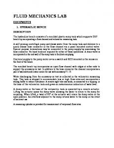
TWO-DIMENSIONAL CAVITY FLOWS Although one cannot experimentally realize genuine two-dimensional (2-D) cavity flows, they are still of interest, because planar flows afford considerable analytical simplification, and their study leads to an understanding of some issues, which is valuable. The visualizations shown in Figure 2 of shear driven flow over rectangular cavities give one an idea of what the flow fields look like; in particular, note the primary eddies that are symmetric about the centerline and the eddies at the corners. We must emphasize, however, that this article deals only with flows driven by boundaries rather than those driven by shear. Even if the planar flow is unsteady, a stream function w exists such that the cartesian components of the velocity are given by u(x, y) 4 ]w/]y, v(x, y) 4 1]w/]x. Note that the vorticity has only one component, x, in the z direction. If the above representations are


96 Figure 2 Experimental visualization of particle paths in shear driven Stokes flows in rectangular cavities. (a) The depth-to-width ratio, $ 4 1/3. Note that only corner eddies are present; (b) $ 4 2. Only one primary eddy is clearly discernable. (From Taneda 1979.)


97

used, the whole field can then be determined, in principle, from the pair of equations for the stream function and vorticity:


¹2w 4 1x,

]x ` (wyxx 1 wxxy) 4 Re11¹2x. ]t

Most of the published literature on 2-D cavity flows deals with a rectangular cavity in which the flow is generated by the steady, uniform motion of one of the walls alone, for example, the lid. This would correspond in Figure 1c to the situation in which there are no end walls to the cavity in the z direction and in which the field is independent of z and t and is generated by the steady, uniform motion of the lid x 4 0 in the y direction as shown. Note that in general the field will depend not only on Re but also on lx, the depth of the cavity; if lx 4 1, the cavity is of square section, the most frequently studied geometry. Here the external length scale has been taken to be Ly, the width of the lid. If we apply the no-slip and impermeability conditions on the side walls and bottom of the cavity and demand that the fluid move with the lid at the lid, there will be a discontinuity in the boundary conditions at the two top corners, where the side walls meet the lid. This is the origin of the so-called corner singularity, which is of theoretical interest but which, not surprisingly, plays but a minor role in the overall field. We postpone for now a discussion of the nature of this singularity.

Stokes Flow To get a feel for the nature of the flow field, it is best to start by looking at the Stokes limit Re 4 0, when the nonlinear inertial terms drop out. It is easy to show that in this limit the stream function now satisfies the biharmonic equation ¹4w 4 0, with w 4 0 on all the walls and with ]w/]n vanishing on the stationary walls and taking the value 11 on the lid. All the early work was based on the numerical solution of the equations resulting from the finite difference formulation of the problem (Kawaguti 1961, Burggraf 1966, Pan & Acrivos 1967). However, for this simple cartesian geometry, it would seem that a series solution based on elementary separable solutions of the biharmonic equation may be feasible. If we take the side walls to be at y 4 51⁄2, the relevant symmetric solutions are of the form e1knx fn(y) where fn 4 y sin kny 1 1⁄2 tan (1⁄2kn) cos kny, and where the eigenvalues kn satisfy the transcendental equation sin kn 4 1kn, all of whose roots are complex. Let {kn, n 4 1, 2, 3.… } be the roots in the first quadrant, ordered by the magnitudes of their real parts; then 1kn, k¯ n, and 1 k¯ n are also roots. The principal eigenvalue k1 is ;4.212 ` 2.251i. One can then attempt to represent the stream function as an infinite sum over these basis functions; that is, w(x, y) 4 5 (n41{anfn(y)e1knx ` bnfn(y)e1kn(lx1x)}, where the unknown complex coefficients {an, bn, n 4 1, 2, 3,… } are determined from the boundary conditions on the lid and the bottom wall alone; the side wall conditions are satisfied exactly by the eigenfunctions. The mathematically inclined reader can see Joseph et al (1982) for some results

98

SHANKAR n DESHPANDE


on the convergence of a biorthogonal series closely related to the above series. It must be noted that, for this non–self-adjoint problem in which all the eigenvalues are complex, there are no obvious orthogonality or biorthogonality relations by which the coefficients can be simply determined. So far, these coefficients have had to be obtained by truncating infinite systems of equations for the unknowns and then solving them for a finite number N of each of the coefficients an and bn. Whereas Joseph & Sturges (1978) generate the infinite system from a biorthogonal series, Shankar (1993) generates the system from a simple least-squares procedure applied directly on the series given above. The latter procedure appears to be more general because it can be carried over, unmodified, to three-dimensional problems. Primary Eddies An idea of the overall eddy structure in the cavity can be obtained from the fields shown in Figure 3 for cavities of depths ranging from 0.25 to 5. One immediately notes that the field consists mainly of a number of counter-rotating eddies. There is but a single primary eddy (PE) when the cavity depth is #1, two eddies when the depth is 2, and four eddies when the depth is 5. In the last case it might be observed that the eddies are similar in shape and almost equally spaced. These features can be easily explained from the form of the eigenfunction expansion for w(x, y) given above. Because the real parts of the eigenvalues kn increase with n, the field for a deep cavity is soon dominated by the principal eigenvalue k1 and can be represented to a very good approximation by the first term of the expansion alone! The x dependence e1(k1r`ik1i)x then indicates that the counter-rotating eddies will be spaced ;p/k1i apart, whereas the field will decay by a factor exp (1pk1r/k1i) in going from one eddy center to the next. This works out to an eddy spacing of ;1.396 and a decay of ;1/357 in the stream function. Although the eddy spacings seen in Figure 3 roughly agree with these ideas, calculations for the infinitely deep cavity (Shankar 1993) verify them to great accuracy. For the latter calculation one need only retain the coefficients an, setting all the bn to zero, reducing the computations by half. We find an infinite sequence of counter-rotating eddies with the properties deduced above. Not only would it be impossible to reach this conclusion by purely numerical means, it is very difficult to make accurate calculations for deep cavities because of the slow penetration of the field into the depths and the large number of grid points required. Corner Eddies and Primary-Eddy Evolution The other important feature of these cavity flow fields is a little less easily seen in Figure 3. At the bottom left and right corners of each cavity are corner eddies, the outer boundary of each being indicated by a w 4 0 streamline. As Moffatt (1964) has shown on very general grounds, we should expect these eddies, driven by the PEs, to exist at the corners. In fact, the theory shows that there should be an infinite sequence of eddies of diminishing size and strength as the corner is approached. Examining Figure 3, which shows a single PE for ,x 4 1 and two for ,x 4 2, a natural


99


Figure 3 The dependence on the depth $ of the 2-D Stokes flow eddy structure in a rectangular cavity. Panels a–e illustrate the effects of increasing depth ($). (From Pan & Acrivos 1967.)


100

SHANKAR n DESHPANDE

question that arises is, ‘‘How does this change in flow topology take place?’’ Accurate calculations show that, when ,x . 1, the corner eddies begin to grow with depth, this growth being very rapid around ,x 4 1.5; moreover, the change in PE topology takes place between depths of 1.6 and 1.7. The relevant changes are shown in Figure 4, in which only one half of the cavity is shown. When ,x 4 1.6295 (Figure 4a), the two corner eddies are still distinct but just touching at the mid-plane. When ,x 4 1.7 (Figure 4b), merger has already taken place with a saddle point in the symmetry plane and with lift off of the first PE. With increasing depth the characteristic cat’s-eye pattern lifts off, becomes weaker, and ultimately disappears, leaving behind the second PE (Figure 4c). Note the growth of the second corner eddy (of the infinite sequence) in this process, which becomes the primary corner eddy after the merger. This process, of the formation of new PEs from the growth and merger of the corner eddies, is repeated indefinitely as the depth is increased. Hellou & Coutanceau (1992) have very skillfully visualized a similar primary-eddy evolutionary process in a different geometry, in which a rotating cylinder drives the motion in a rectangular channel. Corner Singularities We now touch on an issue that is of some theoretical interest, namely the corner singularity issue. To bring the matter into focus, consider the 2-D cavity field formulated above with the lid moving uniformly at unit speed in the y direction. Because the y component of velocity is now required to be 1 on the lid (x 4 0) and 0 on the side walls (y 4 50.5), the boundary condition is discontinuous at the corner; in fact the velocity appears to be bivalued at the corner. With the considerable experience gained from the study of similar problems, for example, in heat conduction in plates with discontinuous boundary conditions and from the Saint-Venant problem in elasticity, one would informally conclude that, whereas the influence of the discontinuity will be increasingly felt as a singular corner is approached, its effect will be negligible over most of the field. Such considerations have led most workers to analyze the field while ignoring the singularity, and the consistency of the results obtained suggests that such

Figure 4 Growth and merger of the corner eddies with increasing cavity depth $ (panels a r c), leading to the formation of the second primary eddy. (From Shankar 1993.)



101

an approach is, by and large, satisfactory. One could avoid this whole issue by making the lid speed continuous but nonuniform in y, such that it vanishes at y 4 50.5, in which case the velocity would be continuous on the whole boundary. But this would amount to the evasion of a genuine issue because an experimental realization of a cavity flow would normally involve a uniformly moving lid. Let us take a more careful look at what is really involved in the corner issue. Let the side wall be of thickness t, and let h be the gap between the moving lid and the top of the side wall. A proper formulation of the problem would now extend the domain to include the gap and permit the specification of no-slip on the top of the side wall and the extended lid and a constant pressure condition, for example, on the external face of the gap. This would make things unambiguous. If h r 0, it seems reasonable to suppose that the field local to the corner must behave as the field local to the corner formed by two rigid planes bounding a viscous fluid, when one of them slides over the other (Batchelor 1967, pp. 224– 26). This can be achieved in a number of ways. Srinivasan (1995) achieves this by writing the stream function as a sum of a singular part with the correct behavior near the corners and a nonsingular part that essentially corrects the contribution of the singular part on the boundaries; a fair amount of numerical work is involved. On the other hand, Meleshko (1996) uses ordinary real Fourier series expansions for the rectangular cavity in a manner such that the required behavior of the field near the singular corners is recovered. The upshot of these studies is what had all along been assumed to be true: the singularities have virtually no effect over most of the flow field, their effects being confined to the neighborhood of the singular corners.

Arbitrary Reynolds Number Once the Reynolds number is allowed to be arbitrary, one has no recourse but to the numerical solution of the governing equations. Thus all the results that we quote below have been obtained by numerical means alone. As has been pointed out earlier for deep cavities, numerical computations can be difficult even for Stokes flow. Naturally, the difficulties increase when nonlinearity is included, particularly as the Reynolds number increases. The resolution of thin shear layers and slow-moving corner eddies and possible new structures in the field all require skill and care. Schreiber & Keller (1983) have pointed out that some of the early 2-D cavity flow computations yielded spurious solutions. The finite-difference equations that are used to approximate the governing field equations will, in general, have a very large complex solution space that may contain more than one real solution vector; it is possible that one may then pick out a spurious real solution. As Schreiber & Keller (1983) convincingly show, mild grid refinements may indicate ‘‘numerical convergence,’’ but possibly to a spurious solution; the physically correct solution may require a very much finer grid. Thus great care and correct technique are required to make reliable and accurate calculations.


102

SHANKAR n DESHPANDE

The Square Cavity Because the lid-driven square cavity (,x 4 1) is now a standard test case for new computational schemes, there are many dozens of papers in the literature that present results with a variety of formulations, numerical schemes, and grids. We mention only Benjamin & Denny (1979), Agarwal (1981), and Ghia et al (1982). All the results that are quoted in this section are from Ghia et al (1982); their results were obtained from a finite-difference form of the stream function-vorticity (w, x) formulation, using uniform cartesian grids. Figure 5 shows the streamline patterns for three Reynolds numbers in a square cavity in which the lid is moving from left to right; note that, for Figures 5–7, the origin is at the bottom left hand corner, and x is to the right. These may be compared with Figure 3c for Stokes flow. For Re 4 100 (Figure 5a), even though the field is no longer symmetric about the mid-plane, it is topologically not different from that in Stokes flow. Initially the center of the PE (where w is a minimum), which was located 0.24 below the lid in the mid-plane, moves a little lower and to the right when Re 4 100. But it is found that, for Re 4 400, the center of the primary eddy has moved lower and back towards the center plane, and, as Figure 5 shows, as Re increases further there is the uniform tendency for the eddy center to move towards the geometric center of the cavity. This can be seen more quantitatively in Figure 6, which shows graphically how the various eddy centers move as Re increases. To facilitate the discussion of the secondary eddies, we designate them bottom right, bottom left, and top left; they are designated BR1, BR2, … , BL1, BL2, . . . , TL1, where the subscripts indicate, except for TL1, the member in a presumably infinite sequence. Recall that the corner eddies were symmetric about the midplane in Stokes flow; as Re increases, although both BR1 and BL1 grow in size, BR1’s growth is greater, as is its strength (as can be seen from the stream function values). The trajectory of the eddy centers is complex, with the distance above the cavity bottom of the center of BL1 being actually greater than that of BR1 for

Figure 5 The dependence on the Reynolds number of 2-D, lid-driven flow in a square cavity; the lid moves from left to right. (a) Re 4 100; the stream function value at the primary eddy centre, wm 4 10.1034; (b) Re 4 1000; wm 4 10.1179; (c) Re 4 10,000; wm 4 10.1197. (From Ghia et al 1982.)



103

Figure 6 The effect of Reynolds number on the location of vortex centers in a square cavity. Here the origin is at the bottom left of the cavity, and x is to the right. (From Ghia et al 1982.)

Re $ 3200. Figures 5 & 6 also show the growth of BR2 and BL2, which are so small and weak in Stokes flow that they have so far not been resolved for the square cavity. The emergence of the upper upstream eddy (UE) (TL1) represents a genuine change in flow topology. Hints of its imminent appearance can be seen in the streamline patterns at Re 4 1000, although it seems to be generally agreed that at this Reynolds number TL1 is absent. Having emerged at a Reynolds number of ;1200 (Benjamin & Denny 1979), it grows in size and strength at least until Re 4 10,000. One must note that this secondary eddy, attached to a plane wall, is quite different in character from the lower-corner eddies; although we have, in agreement with Ghia et al, called it TL1, there is no reason to believe that it is anything other than a single eddy.

104


Figure 7 Vorticity contours in the square, lid-driven cavity. (a) Re 4 100; (b) Re 4 1000; (c) Re 4 10,000. (From Ghia et al 1982.)



105

It should be clear from the above that even the 2-D flow in a cavity of simple geometry can be complex. Although the Stokes flow analysis does provide us with some insight into what might happen, it would be very difficult to even qualitatively predict the changes that are likely to take place as the Reynolds number increases. The vorticity contours of Figure 7 provide insight into some general features of the flow field as the Reynolds number increases. As Re r `, one would expect thin boundary layers to develop along the solid walls, with the central core in almost inviscid motion. This is indeed seen in the figure. As Re increases, there is a clearly visible tendency for the core fluid to move as a solid body with uniform vorticity, in the manner suggested by Batchelor (1956); the calculations show that the core vorticity approaches the theoretical infinite-Re value of 1.886 (Burggraf 1966), with its value being about 1.881 at Re 4 10,000. The vorticity contours show almost circular rings where the gradients in the vorticity are very high and also where they are negligible; clearly great care needs to be exercised to resolve these structures accurately. There appears to be very little work done on deep cavities, although they are of theoretical interest. We would expect a deep cavity to contain a sequence of counter-rotating eddies of diminishing strength and an infinitely deep cavity to contain an infinite number of them. A very natural question is, what happens in a deep cavity when Re r `? We would expect, based on our knowledge of boundary layers and recirculating eddies in channels perhaps, that the first PE will grow in length as some power of Re, most probably the one-half power. Although there is no computational or theoretical work to support this conjecture, Pan & Acrivos (1967) provide some experimental support from measurements in a cavity of depth 10; they find the first PE size to vary as Re ⁄ over the range 1500–4000, beyond which instabilities were found to set in. Some caution has to be exercised, however, because the spanwise aspect ratio of their cavity was only 1, and strong 3-D effects must most likely have been present, as is shown later. Returning to the square cavity, one might wonder about the limit Re r `. There is some computational evidence that the field becomes unsteady around Re 4 13,000. If the flow does become unsteady, what is the nature of this flow, because it cannot, as a 2-D flow, be turbulent? Are there steady solutions that cannot be computed because they are unstable? Although these are natural questions, they are not of practical relevance, because, as we show below, 2-D flows are almost fictitious. So far the discussion has been confined to steady flows in cavities of rectangular section driven by a single moving wall. One can investigate cases in which more than one wall moves (e.g. Kelmanson & Lonsdale 1996), in which the motion is driven by shear rather than by a lid (e.g. Higdon 1985), in which the geometries are different (e.g. Hellou & Coutanceau 1992), and in which the forcing is unsteady (e.g. Leong & Ottino 1989), etc. These will, in general, lead to the introduction of more dimensionless parameters on which the field depends and hence to the possibility of further bifurcations. However, we do not pursue these matters any further because it is usually possible, with the ideas developed above and the general principles put forth in Jeffrey & Sherwood (1980), to 1

2

106

SHANKAR n DESHPANDE

deduce the qualitative behavior of the field in each case, at least at low Reynolds numbers.


THREE-DIMENSIONAL FLOWS The study of 3-D cavity flows is difficult, no matter whether analytical, computational, or experimental techniques are used. In fact hardly any work existed until the pioneering experimental work of Koseff & Street and coworkers at Stanford in the early 1980s. Their studies, however, changed the whole picture because they clearly showed that cavity flows were inherently 3-D in nature. Not only are 2-D models inadequate, they can be seriously misleading. It is worth briefly recalling the nature of the difficulties that one faces in handling these 3-D flows. To start with, analytically one now no longer has a single scalar stream function with which to describe the field; one necessarily has to deal with vector fields, thereby increasing the complexity considerably. A consequence is that, even if we have a precise description of the field, it is difficult to tell whether a given streamline is closed. It may be recalled that, in steady 2D flows, all streamlines are closed except for streamlines that separate eddies by starting and ending on walls. On the other hand, in 3-D flows, closed streamlines are the exception rather than the rule. Computationally, one’s difficulties are compounded by the order-of-magnitude increase in the number of grid points that are required for a given spatial resolution and by the increase in the number of variables and in the complexity of the equations to be solved. Experimentally, the problem manifests itself in the need to accurately describe a fluctuating 3-D field, with little or no symmetry, over the whole cavity. Moreover, there is the difficulty that important flow structures may suddenly appear as the parameters are changed, which can easily be missed if one is not alert. Once the flow becomes turbulent, there are formidable problems in data acquisition, storage, and handling, no matter what technique of investigation is used. We believe that the experience that will be gained in dealing with cavity flows over the next few years will yield strategies to handle unsteady 3-D fields in other branches of fluid mechanics.

Stokes Flow The considerable difficulties posed by 3-D flow fields are already manifest in Stokes flow, where supposedly simple, linear equations hold. The equations that govern the flow field are ¹•u 4 0, ¹p 4 ¹2u. As pointed out earlier, we now no longer have a convenient scalar stream function. It is indicative that we still do not have an analytical or semi-analytical Stokes flow solution for the 3-D flow in a rectangular parallelepiped of the type shown in Figure 1c! If one tries to obtain suitable eigenfunctions from separable solutions to the equations, as was done in the 2-D case, one soon runs into difficulties. These appear to be connected with the new corners that are introduced by the existence of the cavity end walls. It turns out that the natural extension of the 2-D rectangular cavity is to a circular


107


cylinder, rather than a parallelepiped. We therefore consider creeping flow in a cylindrical container generated by the uniform motion of the bottom end wall (Figure 1b) (Shankar 1997). These results are important because they are the only analytical or semianalytical solutions available for a 3-D cavity field.

Flow in a Cylindrical Cavity Let lengths be normalized by the cylinder radius and velocities by the uniform speed of the bottom wall. Let v (r, h, z) 4 e1kz {ƒr(r, h), ƒh (r, h), ƒz (r, h)} be velocity vector eigenfunctions that satisfy the governing equations and the side wall conditions (v 4 0) on r 4 1. It can be shown that, although the h dependences are trigonometric, the radial ones are mixtures of Bessel functions of integer order. It can also be shown that there is a complex sequence {ln} of eigenvalues k as in the 2-D case and a real sequence { kn}, as well. If we now write the velocity field in the cylindrical can as u 4 (anvn, the unknown coefficients an can be found by a least-squares procedure applied to the boundary conditions on the top and bottom end walls of the cylinder in a manner identical to that followed in the 2-D case. Figure 8 shows the streamline patterns in the symmetry plane in cylinders of height 1, 2, 4, and 10, which can be compared to those shown in Figure 3 for the 2-D case. Note that the characteristic length here is the radius of the cylinder and that, in the figure, only one half of the cylinder is shown; the fields are all symmetric about the planes h 4 p/2 and h 4 0. As discussed earlier, the spacing and decay in intensity of the PEs in deep cavities are determined by the principal eigenvalue l1 ' 2.586 ` 1.123i. The PE streamlines look very similar to what were found earlier, at least in the plane h 4 0. But as Figure 9 shows, the corner eddies are very different in nature. Whereas in two dimensions the centers of these eddies are always elliptic points, in three dimensions they can be foci in the plane of symmetry. This can be seen clearly in Figure 9b, in which the streamlines, emanating from the focus on the other side, stream into the focus shown in the figure; note that this would be impossible in two dimensions. Figure 9 also shows the nature of the 3-D streamlines away from the plane of symmetry and the strong azimuthal circulation near the top of the cylinder; the corner eddy is here a truly 3-D object. It may be mentioned that computations show the existence of weaker and smaller second-corner eddies. This is another open problem: what can be said of corner eddies in three dimensions? See Sano & Hasimoto (1980) and Shankar (1998b) for some results on this problem. Three-dimensionality also significantly affects the nature of the corner-eddy merger process that leads to the formation of new primary eddies. It can be seen from Figure 8 that there is one PE when h 4 2, but there are two when h 4 4. We therefore expect the merger process to take place between these two heights. Starting from h 4 3.1, Figure 10 shows the details of this process. Initially there are streamlines flowing into the focus, but soon after, when h 4 3.15, a limit surface S1 exists towards which both the external streamlines and the streamlines from the focus flow. When h 4 3.161 first contact along the top of the can takes


108

SHANKAR n DESHPANDE

Figure 8 Streamlines in a cylindrical container generated by the motion of the bottom end wall. Views are of the plane h 4 0 for containers of heights 1, 2, 4, and 10. Only one half of the symmetry plane is shown in each case. (From Shankar 1997.)

place between the two foci; the limit surface now no longer exists, with all the streamlines flowing out of this focus to the other one along the top of the can. Furthermore, this structure lifts off and metamorphosizes to the second PE with the simultaneous growth of the second corner eddy. Figure 10d shows some 3-D streamlines in the neighborhood of the limit surface, whereas Figure 10e shows some interesting streamlines in the merged region. Note how strong 3-D effects are in these situations. The analysis outlined above can be used to analyze flows in the cylinder generated by more general boundary conditions on the end walls. When symmetry



109

Figure 9 Geometry as in Figure 8 for h 4 2. (a) 3-D streamlines; (b) details of the corner eddy in the plane of symmetry. (From Shankar 1997.)

about the plane h 4 p/2 is broken, very few, if any, of the streamlines are closed (Shankar 1998a).

Steady and Unsteady Laminar Flows: Eddies and Nonuniqueness The Rectangular Cavity It must now be clear that when even the Stokes flow limit poses such problems in 3-D, we have little choice but to resort to computational and experimental techniques to analyze flows at arbitrary Reynolds numbers. Below we deal only with the cavity of uniform rectangular section as shown in Figure 1c and most often where the section is square ($ 4 1); we are not aware of any other 3-D geometries for which any results have been obtained. To simplify matters later, let us define some terms and notation for the cavity geometry shown in Figure 1c. The length scale here is the cavity width Ly in the direction of the moving lid (i.e., ,y 4 1); $ and ! are the dimensionless depth and lateral span, respectively. Thus for the simplest configuration the field depends on the three nondimensional parameters $, !, and Re. Almost all of the published work deals with the cavity of square section $ 4 1. Sticking to tradition, we call (Figure 1c) the 3-D corner eddy bounded by the downstream side


110 Figure 10 Details of the growth and merger of the corner eddy with increasing cylinder height. (a) h 4 3.1; (b,d) h 4 3.15; (c) h 4 3.16; (e) h 4 3.235. (From Shankar 1997.)



111

wall and the bottom wall the downstream secondary eddy (DSE); we call the corresponding eddy between the upstream side wall and the bottom the upstream secondary eddy (USE); and we call the eddy near the top of the upstream wall the upper eddy (UE). The longitudinal vortices bounded by the end walls and the bottom and the end walls and the lid are called end-wall vortices (EWVs). To prevent confusion, all of these have been sketched in the figure. Also shown are sections of certain longitudinal vortices, that is, ones whose axes lie approximately in the streamwise (y) direction, called Taylor-Goertler–like (TGL) vortices. Taken together with the PE in the cavity, we have a rich collection of structures that need to be understood. Although, not much is known about 3-D corner eddies, one would have to keep open the possibility of an infinite sequence of such eddies near the corners. Finally, mention must be made of the starting vortex that develops in the neighborhood of the corner bounded by the downstream side wall and the moving lid. This transient vortex, generated at the impulsive start of the motion, results from the sudden stripping off of the fluid adjacent to the lid by the downstream side wall; it plays no role once the field settles to its asymptotic state. It might help to summarize in advance the changes that take place, for example, in a square cavity of span 3, as Re increases. For low Reynolds numbers (e.g. , 10), the field is qualitatively very similar to that found in Stokes flow with the DSE and USE as secondary flows (with hardly any EWV, if any) in addition to the PE; in the center plane (z 4 !/2), streamlines look similar to those found in 2-D flows, but there are topological differences. Soon after, the lower EWV begins to be evident in the flow, even though very little change occurs in the center plane. As Re increases, initially there are no obvious structural changes, but the asymmetry about y 4 1/2 keeps increasing as do the sizes of the DSE and USE; because the flows are steady, there is symmetry about the mid-plane z 4 !/2. At Re ; 1000, the flow field becomes unsteady with, naturally, loss of symmetry about the mid-plane. Either at this point or soon afterwards, the TGL vortices appear in pairs, taking part in a slow spanwise motion. With further increases in Re, the number of TGL vortex pairs in the cavity increases, and at some stage the UE appears. Finally transition to turbulence in portions of the field takes place at Re ' 6000, with most of the field exhibiting turbulent characteristics when Re 4 10,000. Similar changes take place for cavities of different spans, but naturally the Res at which they take place are different. Velocity Profiles and Particle Trajectories It is only natural to expect the field near the midplane of a cavity of large aspect ratio to be very similar to the field in a 2-D cavity at the same Re. But one should be aware, because of the unavoidable spanwise flow in a 3-D cavity, that the two fields, no matter how similar in appearance, are topologically quite different. Thus in the mid-plane of a 3-D cavity the stagnation points, other than saddles, are usually foci, whereas they are elliptic points in two dimensions. It turns out, however, that the differences are even more significant. The ways in which the horizontal and vertical velocity profiles along the symmetry axes of the mid-plane z 4 !/2 change with Re are


112

SHANKAR n DESHPANDE

Figure 11 Comparison of computed velocity profiles at the mid-sectional plane of a rectangular cavity of span ! 4 3 with the results of 2-D computations. •, – – –, 2-D computations; ––––, 3-D computation. (a) Re 4 10; (b) Re 4 100; (c) Re 4 400; (d) Re 4 1000. Y-axis is along span; see figure 13. (From Chiang et al 1998. Reproduced with permission of John Wiley & Sons Ltd.)

shown in Figure 11 for a square cavity of span 3; also shown are the corresponding 2-D profiles. At Re 4 10 (Figure 11a), the 2-D and 3-D results are almost coincident; this means that for low Res the end walls have almost no effect on the mid-plane field. With increasing Re (Figures 11b–11d), we find boundary layers beginning to form on all the walls and increasing discrepancy between the 2-D and 3-D profiles; because the end walls tend to act as a brake on the fluid, the 3-



113

D velocities tend to be smaller than the corresponding 2-D values. The fact that the discrepancy increases with Re is somewhat counterintuitive, because one might expect that, with decreasing viscosity and thinner boundary layers, the braking action would be less! This point is dealt with a little later. As the span ! is decreased, we would expect the end walls to have a greater effect. That this is indeed so is shown in Figure 12, in which the mid-plane differences are seen to be far larger when the cavity is cubical (! 4 $ 4 1). The 3-D nature of these flow fields is best illustrated by the typical particle tracks shown over half the cavity in Figure 13. Although the flow at Re 4 1500 is mildly unsteady, the tracks shown are very similar to those that would be seen in steady flows at lower Re. Note in particular how, in Figure 13a, a particle starting from just above the bottom plane makes three circuits in the PE before entering the EWV at the end wall, then spirals along the central axis of the cavity to the center plane, and then spirals outwards near this plane before being engulfed in the DSE. This is one of the most important characteristics of three-dimensionality—unlike in two dimensions, the whole cavity is connected! Another feature to be noted is that, in general, the spanwise flow is from the mid-plane to the end walls inside the DSE and the USE and is, to satisfy continuity, in the opposite direction in the core of the PE. With this knowledge of 3-D particle tracks (which are also streamlines in steady flow), we are in a better position to appreciate the projected fields shown in Figure 14. Each frame includes three planes on which the projections of certain nearby streamlines are shown; of course, by symmetry the lines shown on the mid-plane z 4 !/2 are the streamlines themselves. These figures clearly show (a) how three-dimensionality modifies the fields near the

Figure 12 Comparison of velocity profiles at the mid-sectional plane of a cubic cavity with 2-D results; Re 4 1000. M, 3-D computation; ––––, 2-D computation. (From Ku et al 1987.)


114 Figure 13 Three-dimensional particle paths in a lid-driven rectangular cavity. Only a half of the cavity is shown, with the mid-plane to the left in each case. ! 4 3; Re 4 1500. (From Chiang et al 1996. Reproduced with permission of John Wiley & Sons Ltd.)



(a)

(b)

115

(c)

Figure 14 The projections of the streamlines onto the end walls, side walls, and midplanes of the lid-driven cubic cavity. The lid moves in the y direction. (a) Re 4 100; (b) Re 4 400; (c) Re 4 1000. (From Iwatsu et al 1989.)

mid-plane and the end walls and near the plane y 4 1/2 and the side walls, (b) how the build up of the central recirculation with Re is connected with the stronger swirl near the end walls, and (c) how, while the lower EWVs appear at moderately low Re and seem to span the width of the cavity, the upper EWVs appear later and do not span the whole width. Note also, as pointed out earlier, that, unlike in two dimensions, stagnation points other than saddles are usually foci rather than elliptic centers; moreover, streamlines are usually not closed. We return to the somewhat puzzling fact that the center-plane velocity profiles are coincident with their 2-D counterparts at low rather than high Re. The explanation lies in Figure 15, which shows the effect of Re on the projections of the streamlines through the plane y 4 0.525 on that plane. At Re 4 1 (Figure 15a), the spanwise velocities are negligible, and the EWVs can hardly be resolved, even if present; although not shown here, at Re 4 10, there are significant spanwise motions near the bottom and top walls but still no discernable EWVs. When Re 4 50 (Figure 15b), the lower EWV is clearly evident, whereas it is only at Re 4 ;100 (Figure 15c) that the upper EWV can be identified. These panels clearly show that the spanwise flow, which is negligible at low Re, becomes increasingly important as Re increases. Thus the boundary-layer effect and this 3-D effect are in competition as Re increases, and the latter effect ultimately


116 Figure 15 Projections of the streamlines onto the plane y 4 0.525, showing the development of the end wall vortices with increasing Reynolds number. (a) Re 4 1; (b) Re 4 50; (c) Re 4 100. (From Chiang et al 1998. Reproduced with permission of John Wiley & Sons Ltd.)


117


dominates; in fact, to such an extent that, although there is no spanwise flow midplane, the velocity profiles there deviate from the corresponding 2-D profiles. Poincare´ Sections A characteristic feature of 3-D streamlines has already been pointed out—that in general they do not close, not even in mid-plane. Consequently, one may expect that, even in steady flows with considerable symmetry in the driving conditions, individual particles in the fluid may move in apparently complicated paths over a considerable portion of the cavity. Whereas particle paths such as those shown in Figure 13 are illustrative of this facet of the motion, another way of examining this issue is to look at Poincare´ sections, as shown in Figure 16. These have been obtained (Ishii & Iwatsu 1989) by tracking a number of particles in a cubic cavity and marking with a point each time a particle path intersects the plane y 4 1/2; thus, each frame in the figure shows the points at which the streamlines generated by a number of distinct tracer particles have intersected this plane many times. We see in Figure 16a, at Re 4 100, four distinct patches; the two upper patches correspond to motion into the plane, whereas the lower ones correspond to motion out of the plane; for particles started symmetrically and in synchronization, the two left patches should be identical to the two right patches because the motion is symmetric about the mid-plane. Note that each patch contains a central point immediately surrounded by a set of five points that seem to lie on some closed curve; these points are further surrounded by four sets of points each apparently lying on a well-defined closed curve; finally all of these are surrounded by a large number of points lying apparently at random in an annular region. What is very interesting is that these sections strongly suggest the existence of closed streamlines that lie on tori; the single point in a patch is of period 1, the set of 5 points in a patch of period 5, and so on. The outermost annular ring suggests a motion that is not on a torus and is probably not periodic at all (i.e. the streamline is not closed). The situation is far more complicated at Re 4 200, where possible islands of closed streamlines of more complex shape are again surrounded by regions of possibly nonperiodic orbits. The complexity increases until, at Re 4 400, it is hard to visualize any closed orbits (streamlines). It must be emphasized (a) that no numerical technique can ever be used with certainty to pick closed orbits, (b) that these flows are steady, laminar flows, and (c) that the apparently chaotic behavior (sometimes called Lagrangian chaos) of the tracer particles is caused, not by the nonlinearity of the N-S equations, but by that of the (Lagrangian) particle path equations. This cannot happen in steady, 2D flow, because, even though the equations are still nonlinear, the system is integrable. Taylor-Goertler–Like Vortices With an increase of Reynolds number, at some stage, depending on the aspect ratio !, two new features appear, longitudinal vortices and the upstream upper eddy; the latter appears later, after the flow has become unsteady, and both seem to remain well into transition to turbulence and later. The longitudinal vortices (see Figure 17), whose axes lie along the primaryflow direction, were first identified in their experiments and named Taylor-


118

SHANKAR n DESHPANDE

Figure 16 Poincare´ sections of streamlines in the plane y 4 0.5. (a) Re 4 100; (b) Re 4 200; (c) Re 4 300; (d) Re 4 400. (From Ishii & Iwatsu 1989.)

Goertler–like (TGL) vortices by Koseff & Street (1984a,b,c). The rationale for the name is that these vortices bear a strong resemblance to the longitudinal vortices that arise from centrifugal instability in flows along concavely curved walls. The analogy is somewhat imperfect here because the concavely curved separation surface between the PE and the DSE is not a solid wall; however, there is experimental evidence that this surface is indeed the source of instability. For a a linear-stability analysis based on 3-D perturbations to 2-D base flows, see



119

Figure 17 Flow visualization of Taylor-Goertler–like (TGL) vortices. Views from the downstream side wall of TGL vortex pairs along the bottom wall. $ 4 1; ! 4 3. (a) Re 4 3300; (b) Re 4 6000. (From Rhee et al 1984.)

Ramanan & Homsy (1994). Aidun et al (1991) have identified the stages by which the TGL vortices appear for ! 4 3. The flow is steady up to around Re 4 825; a little beyond, small amplitude, time-periodic waves appear on the DSE. Pairs of vortices, generated near the mid-plane, move towards the end planes with a corkscrewing motion. With increasing Re, there is a slight decrease in the period of the oscillations ('3 s) until, at Re 4 1000, there is a second transition in which the boundary between the DSE and the PE becomes irregular, with the wave motion traveling towards the end walls featuring discrete vertical spikes. According to the authors these spikes grow crowns at their tops, giving them a mushroomlike appearance, and these shapes are what are seen at the side walls, as in Figure 17, and are identified as TGL vortex pairs. The unsteady, longitudinal nature of these formations in a cubical cavity at Re 4 4000 has also been verified in the computations of Iwatsu et al (1989). It seems to be generally agreed that the number of pairs of TGL vortices, which is six soon after inception for ! 4 3, increases with Re, being 8 at Re 4 3000 and 11 at Re 4 6000 (Koseff &


120

SHANKAR n DESHPANDE

Street 1984a). These interesting structures seem to persist even after the flow has become turbulent. A brief word of caution regarding so-called ‘‘separation surfaces’’ is in order here. In 2-D, the primary eddies and secondary eddies are, in steady flow, isolated from one another by separation surfaces; fluid particles cannot cross these surfaces, and, as a consequence, there is no mixing between the various eddy structures. This does not hold in 3-D, as can be seen clearly, for example, from Figure 13. Fluid particles can move from structure to structure, in a sense globalizing the flow, and so the nature of the ‘‘separation surfaces’’ in the fluid is very much more complex and is not easy to define. The reader should also be aware that, in some of the literature, closed streamlines, clearly defined ‘‘separation surfaces,’’ etc, are sometimes sketched (as in Figure 1c), which are likely to be erroneous. These errors arise out of a desire to understand, in simple 2-D terms, genuinely complex 3-D flows. Some indication of the quantitative differences between 2-D cavity flows and the mid-plane fields in 3-D cavities is given in Figure 18. As far as the DSE size is concerned, it is seen that, whereas for a cavity with ! 4 3 the growth trend with Re is similar to that found from 2-D computations, if ! 4 1 then even the trend is wrong. But, even with ! 4 3, the mean velocity profiles along the symmetry axes at mid-plane are very different from the computed 2-D profiles (Figure 18b). As explained earlier, the drag of the end walls tends to act as a brake, and so the peaks are smaller in 3-D. At first sight it may appear surprising that even a span of three is inadequate to ensure 2-D flow at the mid-plane. But on reflection it is clear that, the braking effect of the end walls aside, the very existence of the TGL vortices for sufficiently large Re and ! implies that it is virtually impossible to obtain a truly 2-D flow in such cavities, no matter how large ! is and no matter how far away the end walls are. This fact has been stressed by the Stanford group. Solution Multiplicity The uniqueness of steady flows is almost an article of faith for most of us; for a given geometry and forcing, the field must be unique. Cavity flows provide interesting counter examples to shake this belief! Aidun et al (1991) have found that, in a lid-driven cavity (! 4 3), if the lid suddenly decelerates the flow from Re ' 2000 to Re ' 500, the original PE state may or may not recover. In its place steady cellular patterns may stabilize. Aidun et al (1991) have identified three other states, having 2, 3, and 4 cells, all symmetric about the mid-plane, whose end views (as seen from the downstream side wall) are shown in Figure 19a. Thus, although for Re r 0 there is a unique (Stokes) flow field, for sufficiently large Re the field obtained by Reynolds number continuation from this is apparently not unique. Aidun et al point out a possible technological implication in the coating industry. It is known that short-dwell coaters (Figure 1a) do not always behave the same way under identical operating conditions; they suggest that this may be caused by the multiplicity of the permissible flow states. Three-dimensional computational confirmation of these multiple solutions is as yet unavailable. Kuhlmann et al (1997) provide another example of multiple solutions. The geometry considered is a rectangular cavity


121

(a)

(b)

Figure 18 Comparison of experimental data for a lid-driven cavity ($ 4 1), with the results of 2-D computations. (a) Downstream eddy size as a function of Reynolds number. ., ! 4 3; ,, ! 4 1. Experimental, •, 2-D computations. (b) Velocity profiles in the symmetry plane, Re 4 3200. D, Experimental (! 4 3); ––––, 2-D computations. (From Koseff & Street 1984a,c.)


122 (b) Figure 19 Stable multiple solutions in driven cavity flow. (a) Flow visualizations from the downstream side wall of two-cell, three-cell, and four-cell steady states (from Aidun et al 1991); (b) shear stress x ; Re in a double lid-driven cavity, indicating two stable states between Re(01) 4 234.3 and Re(0`) 4 427. (From Kuhlmann et al 1997)


123


with a pair of opposite walls moving at the same speed in opposite directions. As might be expected, the basic state (called ‘‘two-vortex flow’’ by the authors) at low Re consists of a pair of corotating vortices, attached one each to each moving wall. Two-dimensional calculations (for $ 4 1.96), based on Reynolds number continuation, show that, although this state does not exist beyond Re ' 427, another 2-D solution state (called ‘‘cat’s-eye flow’’ by the authors) does exit. As Figure 19b shows for 235 , Re , 427, there exist two solutions stable to 2-D disturbances, and one that is unstable. The nice feature here is that Kuhlmann et al were able to show in experimental (3-D) simulations of the field that both states could be realized in the laboratory. As Re is gradually increased, the initial field corresponds to the two-vortex flow state; at Re ' 232 there is a jump transition to the cat’s-eye flow state. When Re is gradually reduced, the flow switches back from the cat’s-eye to the two-vortex state at Re ' 224, exhibiting hysteresis and solution multiplicity. A full 3-D simulation of this field too would be of interest.

Transitional and Turbulent Flows as Deduced from Experiments and Direct Numerical Simulations Although most fluid dynamicists believe that turbulence is contained in the N-S equations, strong computational evidence to support this belief has until recently been lacking. One of the most valuable results of research in the area of driven cavity flows has been the generation of such evidence. As pointed out earlier, the simple geometry and unambiguous boundary conditions facilitate the direct, reliable comparison of experimental data with DNS. The importance of this feature for turbulent flows can only grow in the future as simulations at higher Re become feasible. As with any other 3-D flow, once Re is sufficiently high the flow in a cavity will become transitional and then evolve into turbulent flow. In this section we consider only the lid-driven cavity of constant square section ($ 4 1) because this is the only cavity for which detailed measurements and computations have so far been carried out. A summary scenario valid for 1 # ! # 3 is as follows. The fields are generally unsteady laminar flows for Re up to ;6000; transition, meaning transition to turbulence, takes place in the range 6000 , Re , 8000, and sufficient portions of the fields are turbulent by Re 4 10,000 for them to be called turbulent flows. Attention needs to be drawn to certain features of transition and turbulence in driven cavity flows that are somewhat special. First of all, the fluid field is usually already unsteady with, for example, the TGL vortices before transition to turbulence. Transition appears initially to take place in the region of the DSE (Koseff & Street 1984a), while the rest of the field is still laminar. With increasing Re, the flow becomes turbulent, perhaps first in the region of the DSE and then gradually over most of the cavity. The fact that different parts of the field, such as the regions close to the moving wall, near the DSE and USE, in the core, etc, can be in different states (laminar, transitional, or soft or hard turbulent)


124

SHANKAR n DESHPANDE

adds to the difficulty in understanding these complex flows. This is particularly true at the lower Reynolds numbers that we are considering (Re # 10,000) Although we have no intention here of addressing the difficult question of how one can decide whether the field at a point (or in the neighborhood of a point) is turbulent, it might help nonspecialists to consider this issue. How does one decide whether the velocity at a point is characteristic of a locally turbulent flow? The position taken here is that, if the field is locally turbulent, (a) the velocity component traces will have the appearance of being random, (b) the velocity components will not be highly correlated in time, (c) the power spectra of the signals will have that characteristic of turbulent fields (low-frequency peak and an inertial subrange followed by a high-frequency dissipation range). Figure 20 shows two sets of experimentally obtained unsteady u and v time traces at two Reynolds numbers. At Re 4 3200 (Figure 20a), although both signals display large variations, the signal lengths are insufficient to even casually determine ‘‘randomness’’; it is obvious that u and v are strongly correlated, and this indicates a nonturbulent field, which the spectrum (not shown here) corroborates. On the other hand, at Re 4 10,000 (Figure 20b), both signals have a noisy, random appearance; they do not appear to be well correlated, which calculations confirm; and the spectra do turn out to be characteristic of turbulent flows. We therefore conclude that the point under consideration is in a turbulent field. A minor but interesting issue is the source of the large amplitude fluctuations seen in Figure 20a. Prasad & Koseff (1989) point out that these are caused by the to and fro ‘‘meanderings’’ of the two pairs of TGL vortices that are at the bottom of the cubic cavity; the period is approximately 3 min. It should be pointed out that, computationally, (a) Perng & Street (1989) resolved nonstationary TGL vortices for Re 4 3200, but their assumption of symmetry about the mid-plane can be criticized; (b) Iwatsu et al (1990) found two stationary pairs of TGL vortices at Re 4 2000, whereas (c) the computations of Chiang et al (1996) for Re 4 1500 and ! 4 3 show that the TGL vortices rise at midspan and drift to the end walls. So it seems more likely that it is the drifting past of newly formed TGL vortices, rather than the meandering of the same vortices, that causes the excursions seen in the traces. It also appears that the TGL vortices continue to be part of the field even after the transition process starts, and it is only after the field becomes strongly turbulent that random momentum transport tends to destroy these surprisingly rugged structures. One therefore expects to see a gradual transition from a TGL-dominated to a turbulence-dominated field. Turbulence in the Cubic Cavity For economy, we combine the description of the time-averaged velocity field in a lid-driven cubic cavity at Re 4 10,000 with the comparison of the results obtained for this geometry from experiments with results from DNS (Deshpande & Shankar 1994a,b; Verstappen & Veldman 1994). The experimental data were obtained (Prasad & Koseff 1989) by using a standard laser-Doppler system in a belt-driven cavity; valuable experimental data for other aspect ratios (! 4 0.5 and 3) are available in Prasad & Koseff (1989) and Koseff

(b)

Figure 20 Velocity-time traces at points close to the bottom wall of a lid-driven cavity flow. $ 4 ! 4 1. (a) Re 4 3200; (b) Re 4 10,000. (From Prasad & Koseff 1989.)

125


(a)

126

SHANKAR n DESHPANDE


& Street (1984c). Regarding DNS, it must be remembered that no modeling whatsoever is involved here, because the N-S equations are solved directly; if there are no errors in discretization and if the solutions of the discretized equations can be assumed to approximate the solutions of the N-S equations, only the adequacy of the spatial and temporal resolution can be seriously questioned. We return briefly to this issue later. We begin by observing how the mean velocity components along the symmetry axes in mid-plane (z 4 0.5) vary as the flow shifts from steady laminar to unsteady laminar to turbulent flow (Figure 21); as usual, we write v 4 v¯ ` v8, where v¯ and v8 are the mean and fluctuating parts of v etc. As might be expected, near the lid the streamwise v¯ component displays a steadily thinner boundary

Figure 21 The variation with Re of time-averaged velocity profiles on different centerlines in a cubic cavity. Also shown are the experimental results for Re 4 3200 (V). (a) Line y 4 z 4 0.5; (b) line x 4 z 4 0.5; (c) line x 4 y 4 0.5; (d) line x 4 y 4 0.5. (d from Deshpande et al 1994; the rest are from Deshpande & Milton 1998.)



127

layer as Re changes from 1000 to 10,000. But at the bottom wall, counterintuitively, the peak v¯ decreases with Re although it does move towards the wall as expected. Although the decrease of the peak from 1000 to 3200 is principally caused by 3-D effects, the decrease from 3200 to 10,000 is influenced considerably by the turbulent nature of the flow; note that, in the turbulent flow, the core is much more energetic, presumably owing to turbulent transport from the wall layer. A similar behavior is seen for the downward u¯ component in Figure 21b. The figure also shows the profiles obtained experimentally for Re 4 3200, which compare well with the simulations for that Re. In Figure 21c,d are displayed the mean components along the line normal to the mid-plane and passing through its center. We would expect the steady laminar flow and the mean unsteady flows to be symmetric about the mid-plane (z 4 0.5). The figures clearly bear this out for Re 4 1000 and for the unsteady flow at Re 4 3200. For the turbulent flow at Re 4 10,000, reasonable symmetry has been achieved for the spanwise w component; but in Figure 21d the fact that u¯ has yet to achieve symmetry implies that the length of the trace over which the averaging has been done is somewhat too small. It is pointed out in Deshpande et al (1994) that the problem of achieving this symmetry is even more severe for the turbulent stresses. On the positive side one can look on this characteristic as one more possible check on the level of reliability of the calculations. Coming to the comparison of the turbulent field obtained by DNS with that obtained experimentally at Re 4 10,000, Figure 22 shows the components of the mean velocity along the symmetry axes of the mid-plane. Although the streamwise components compare quite well over the whole range, the downward components agree well everywhere except near the downstream side wall, where there is a mismatch of peaks of almost 25%. Note that there is some indication that the

Figure 22 Mean velocity profiles along the symmetry axes, mid-plane in a lid-driven cubic cavity. Re 4 10,000. V, Experiments, Prasad & Koseff (1989); ––––, direct numerical simulation results, Deshpande & Shankar (1994b); – – –, 2-D results, Ghia et al (1982).

128

SHANKAR n DESHPANDE


mean spanwise vorticity in the core is approximately uniform. Also shown in the figure are the results of steady, laminar, 2-D computations that show that these cannot reasonably simulate the mean turbulent field even at the cavity mid-plane; the comparisons are not much better even with experimental results for a cavity with ! 4 3. The comparisons of turbulent stresses are shown in Figure 23. Although the quantitative agreement here is not as good as for the mean-velocity components, the general qualitative agreement is encouraging; the agreement is

Figure 23 Turbulent stresses along the symmetry axes, mid-plane in a lid-driven cubic cavity. Re 4 10,000. V Experiments, Prasad & Koseff (1989), –––– DNS results, Deshpande & Shankar (1994).


129

COMPUTATION EXPERIMENT

3

–2

10

5 10–3

10–4 MAGNITUDE


best for urms, in which even the peaks near the side walls are captured adequately. The data reveal some interesting features of the turbulent field. The rms velocity and the Reynolds stress are an order of magnitude larger near the downstream wall than near the upstream wall, whereas the peak magnitudes near the bottom wall appear to lie between those at the side walls. This seems to suggest that, in this recirculating flow, the fluctuations are largest near the downstream side wall, that they reduce in intensity along the bottom wall, and that they further reduce in intensity in the generally accelerating flow in the neighborhood of the upstream side wall; in fact, there could well be regions where relaminarization takes place. It was pointed out earlier that one of the indicators for turbulence is the nature of the power spectrum of the velocity components. Figure 24 shows the v8 power spectra obtained experimentally and computationally at a point near the bottom

10–5

10–6

10–7

10–8 0.01

0.1

1

FREQUENCY

Figure 24 Comparison of the computed and experimentally obtained v8 power spectra at the point (0.966,0.5,0.5) in a cubic cavity. Re 4 10,000. (From Deshpande & Shankar 1994b.)

130

SHANKAR n DESHPANDE


wall, at mid-plane. It must be mentioned that there are technical difficulties, discussed in Deshpande & Shankar (1994a), in obtaining and comparing these spectra, which stem from the finite length of the signal traces, the averaging procedures used to smooth the highly oscillatory raw spectra, etc; we only briefly discuss these points here, first noting that there is reasonable agreement between the two spectra, in keeping with the agreement found earlier between the two fields at mid-plane. Of greater interest is the fact that the characteristics of both spectra are not in conflict with the expected characteristics of turbulent signals at high Re: a flat low-frequency peak, an inertial subrange with a roughly 15/3rds slope, followed by a rapid high frequency decay to the dissipation range. It is true that the inertial subrange hardly spans a decade and that it would have been more comforting if this range had been larger. Although there seems to be no doubt about the flow being turbulent, we are probably dealing here with soft turbulence, at an Re too low to fully mimic classical turbulence. There will be great interest in extending these investigations to higher Re.

Kolmogorov Scales in the Cavity A notion that has proved to be useful in the study of turbulence is that of the energy cascade. The turbulent fluctuations are considered to be driven by the mean flow, with the energy being transferred, principally by inviscid interactions, from large scales to small scales in the form of a cascade, with dissipation occurring at the smallest scales, the so-called Kolmogorov scales. One of the advantages of DNS is that the detailed knowledge of the field provides us an opportunity to examine where dissipation takes place and how the Kolmogorov scales are distributed over the field. The dimensionless dissipation function f(x, t) is given by f 4 [(]ui /]xj) ` (]uj /]xi)]2; the instantaneous dimensional total dissipation rate per unit mass will then be vfV 20 /L y2. Now f can be written as the sum of terms coming from the mean velocity components (fm), the fluctuating components (ff ), and the interaction of the two (fmf ). Because the time average of fmf is zero, the time average of f, f is given by f 4 fm ` ff. The time traces of f at four depths along the vertical center line in the mid-plane of the cavity are shown in Figure 25. We note (a) at x ' 0.02, the point closest to the moving lid, both the dissipation and the amplitude of its fluctuations are large; (b) at the next point (x ' 0.07), close by, both the mean and the amplitude of the fluctuations have dropped sharply, but the frequency of the oscillations has increased perceptably; (c) at the point close to the primary vortex center (Figure 25c), there are prolonged periods of low dissipation followed by periods of activity, at levels at times higher than at the previous point; and (d) at the bottommost point, the intermittency has disappeared whereas the peaks have increased. Deshpande & Milton (1998) point out that most of the contribution to the time-average dissipation f comes from fƒ rather than from fm; that is, it is the fluctuations that contribute mainly to the mean dissipation. This result is known to be true for turbulent flows at high Re, away from the walls, but it is interesting to find that it holds even at Re 4 10,000. Thus even



131

Figure 25 Time traces of the total dissipation function f on the line y 4 z 4 0.5, at different x values. Re 4 10,000. (From Deshpande & Milton 1998.)

at this low Re, the turbulent cavity flow displays an important feature characteristic of high Re turbulent flows. The Kolmogorov microscales are the smallest scales supported in a turbulent flow. Apart from its fundamental importance, a knowledge of the actual distribution of these scales in the field will help, despite certain philosophical and logical problems, in planning further direct numerical simulations and estimating the adequacy of the resolution obtained. The Kolmogorov microscales depend on the rate of dissipation and the kinematic viscosity. Let e 4 fƒ /Re be the dimensionless dissipation rate, and let gk be the Kolmogorov length scale nondimensionalized by Ly, the cavity width. Then, for example, gk 4 (1/eRe3)0.25 4 (1/fRe2)0.25. It must be noted that, because nine velocity derivatives need to be evaluated, it is very difficult to experimentally determine gk even at a few points in the field. The power of DNS can be seen here, because it can be used to determine the distribution of e and gk over the whole domain. Figure 26 shows the distribution of gk along the vertical and horizontal lines of symmetry on five z planes. The distributions are roughly similar in the four planes other than the one closest to the end wall (z ' 0.006). In these four planes, gk is smaller at the walls than near the primary vortex center, the smaller value indicating a higher rate of dissipation and turbulence activity. The profiles near the end walls are more uniform, with corresponding indications for dissipation and turbulence


132

SHANKAR n DESHPANDE

Figure 26 Profiles of the Kolmogorov length scale gk in different z planes. (a) Along the line y 4 0.5; (b) along the line x 4 0.5. (From Deshpande & Milton 1998.)

activity. We also observe that, away from the end walls, there are large gradients in gk near the lid and the downstream side wall. It is also found, not surprisingly, that turbulence activity is more vigorous near the DSE than near the USE. Some words of caution regarding the above Kolmogorov scale calculations and some comments regarding DNS are appropriate here. First, gk comes from a scaling argument, and in its evaluation from e the constant of proportionality is bound to remain unknown. It is generally believed that, to simulate a turbulent flow directly, the Kolmogorov scales have to be resolved. It should be kept in mind, however, that these scales are evaluated by summing nine velocity derivatives and averaging over time, and hence they are a representation of the smallest scales at a particular point in a stationary turbulent flow, in a statistical sense only. Thus spatial scales smaller than gk are bound to occur at this point for some shorter durations. It is generally believed (Reynolds 1990) that the number of grid points required scales with Re9/4; hence, for given computing power there is an upper limit to the Reynolds number that can be achieved. Many DNS calculations, for example the ones cited here, seem to be reasonably good (in the sense shown above) even though they do not resolve the smallest scales. This is probably because the smallest scales are not dynamically very important as far as the overall field is concerned. We describe an analogy of sorts: in 2-D cavity flows, we are unable to resolve the infinite sequence of corner eddies, sometimes not more than one, yet we still get reasonable results for the overall field. This is not to deny the importance of fine grids in simulation or the existence of the high Re limit; the point is that, perhaps, while being careful, one need not be too conservative. The grid resolution and the averaging time required depend on the quantity of interest (mean velocity, rms values, shear stresses, or higher moments). The distribution of gk in the cavity also indicates the difficulty of selecting a good grid for a 3-D simulation; unstructured grids may be advantageous in this regard.



133

Finally, as an interesting exercise we compare the exact value of dissipation computed above with that obtained by an inviscid estimate from GI Taylor. In this estimate the dissipation is equal to Au3/l (Tennekes & Lumley 1972, p. 20), where u is the characteristic velocity of fluctuation, l is an integral length scale, and A is a constant of proportionality. Taking u to be the average of the three rms values and l 4 ly 4 1, if we now compare this inviscid estimate with the exact value of the dissipation, we can estimate A. If the inviscid estimate is reasonable, we should find little variation in A, and with luck it may even be close to 1. This interesting comparison was made by Deshpande & Milton (1998), who find that the inviscid estimate is quite good over the bulk of the flow, away from the walls and the DSE. Many other investigations are possible with DNS. For example, it is possible to show that the initial state of the fluid in the cavity does not influence the final turbulent state (Milton & Deshpande 1996), to put bounds on when transition takes place, etc. Work has already been initiated (Zang et al 1993, Jordan & Ragab 1994) in using 3-D cavity flows to study and improve LES models. But these matters would take us too far afield.

CONCLUSION Over the past nearly four decades the study of driven cavity flows has lead to insights into various aspects of fluid mechanics, some of them counter intuitive and at times controversial. It may be noted from the literature cited that the pace of work in the field has accelerated in recent years, principally because of the possibilities opened up by DNS. In our opinion this growth is going to continue because of the importance, both theoretical and practical, of being able to analyze and understand complex, 3-D turbulent flows. A bottleneck that we do see is the paucity of experimental data that are available. Extending the work of the Stanford group to map a greater part of the field and to higher Reynolds numbers is a matter of real importance. Although there are still many issues at lower Reynolds numbers that are important and of interest, the understanding of high-Reynoldsnumber flows is paramount. We expect DNS to play an increasingly important role in this endeavor.

ACKNOWLEDGMENT We thank S. Nagendra for help with the figures. We also acknowledge with gratitude the support of the Aeronautical Research & Development Board for our own cavity flow work and the National Aerospace Laboratories for its support over all these years. Visit the Annual Reviews home page at www.AnnualReviews.org.

134

SHANKAR n DESHPANDE


LITERATURE CITED Agarwal RK. 1981. A third-order-accurate upwind scheme for Navier-Stokes solutions at high Reynolds numbers. AIAA Pap. No. 81-0112 Aidun CK, Triantafillopoulos NG, Benson JD. 1991. Global stability of a lid-driven cavity with through flow: flow visualization studies. Phys. Fluids A 3:2081–91 Batchelor GK. 1956. On steady laminar flow with closed streamlines at large Reynolds numbers. J. Fluid Mech. 1:177–90 Batchelor GK. 1967. An Introduction to Fluid Dynamics. Cambridge, UK: Cambridge Univ. Press Benjamin AS, Denny VE. 1979. On the convergence of numerical solutions for 2-D flows in a cavity at large Re. J. Comput. Phys. 33:340–58 Bogatyrev VYA, Gorin AV. 1978. End effects in rectangular cavities. Fluid Mech.-Soviet Res. 7:101–6 Burggraf OR. 1966. Analytical and numerical studies of the structure of steady separated flows. J. Fluid Mech. 24:113–51 Chiang TP, Sheu WH, Hwang RR. 1996. Finite volume analysis of spiral motion in a rectangular lid-driven cavity. Int. J. Numer. Meth. Fluids 23:325–46 Chiang TP, Sheu WH, Hwang RR. 1998. Effect of Reynolds number on the eddy structure in a lid-driven cavity. Int. J. Numer. Meth. Fluids 26:557–79 Deshpande MD, Milton SG. 1998. Kolmogorov scales in a driven cavity flow. Fluid Dyn. Res. 22:359–81 Deshpande MD, Milton SG, Balaji S. 1994. A detailed description of transitional and turbulent flow in a three-dimensional cavity. Natl. Aerosp. Lab. Doc. PD CF 9430. Bangalore, India: Natl. Aerosp. Lab. Deshpande MD, Shankar PN. 1994a. Direct numerical simulation of a complex turbulent flow. Curr. Sci. 66:767–70

Deshpande MD, Shankar PN. 1994b. Transitional and turbulent flow in a three-dimensional cavity. Natl. Aerosp. Lab. Doc. PD CF 9411. Bangalore, India: Natl. Aerosp. Lab. Ghia U, Ghia KN, Shin CT. 1982. High-Re solutions for incompressible flow using the Navier-Stokes equations and a multigrid method. J. Comput. Phys. 48:387–411 Hellou M, Coutanceau M. 1992. Cellular Stokes flow induced by rotation of a cylinder in a closed channel. J. Fluid Mech. 236:557–77 Higdon JJL. 1985. Stokes flow in arbitrary two-dimensional domains: shear flow over ridges and cavities. J. Fluid Mech. 159:195–226 Ishii K, Iwatsu R. 1989. Numerical simulation of the Lagrangian flow structure in a drivencavity. In Topological Fluid Mechanics, ed. HK Moffatt, A Tsinobar, pp. 54–63. Cambridge, UK: Cambridge Univ. Press Iwatsu R, Hyun JM, Kuwahara K. 1990. Analyses of three-dimensional flow calculations in a driven cavity. Fluid Dyn. Res. 6:91– 102 Iwatsu R, Ishii K, Kawamura T, Kuwahara K, Hyun JM. 1989. Simulation of transition to turbulence in a cubic cavity. AIAA Pap. No. 98-0040 Jeffrey DJ, Sherwood JD. 1980. Streamline patterns and eddies in low-Reynolds-number flow. J. Fluid Mech. 96:315–34 Jordan SA, Ragab SA. 1994. On the unsteady and turbulent characteristics of the threedimensional cavity flow. J. Fluids Eng. 116:439–49 Joseph DD, Sturges L. 1978. The convergence of biorthogonal series for biharmonic and Stokes flow edge problems, part II. SIAM J. Appl. Math. 34:7–26 Joseph DD, Sturges LD, Warner WH. 1982. Convergence of biorthogonal series of biharmonic eigenfunctions by the method


FLUID MECHANICS IN THE DRIVEN CAVITY of Titchmarsh. Arch. Ration. Mech. Anal. 78:223–74 Kawaguti M. 1961. Numerical solution of the the Navier-Stokes equations for the flow in a two-dimensional cavity. J. Phys. Soc. Jpn. 16:2307–15 Kelmanson MA, Lonsdale B. 1996. Eddy genesis in the double-lid-driven cavity. Q. J. Mech. Appl. Math. 49:635–55 Koseff JR, Street RL. 1984a. Visualization of a shear driven three-dimensional recirculating flow. J. Fluids Eng. 106:21–29 Koseff JR, Street RL. 1984b. On the endwall effects in a lid-driven cavity flow. J. Fluids Eng. 106:385–89 Koseff JR, Street RL. 1984c. The lid-driven cavity flow: a synthesis of qualitative and quantitative observations. J. Fluids Eng. 106:390–98 Ku HC, Hirsh RS, Taylor TD. 1987. A pseudospectral method for solution of the threedimensional incompressible Navier-Stokes equations. J. Comput. Phys. 70:439–62 Kuhlmann HC, Wanschura M, Rath HJ. 1997. Flow in two-sided lid-driven cavities: nonuniqueness, instabilities and cellular structures. J. Fluid Mech. 336:267–99 Leong CW, Ottino JM. 1989. Experiments on mixing due to chaotic advection in a cavity. J. Fluid Mech. 209:463–99 Meleshko VV. 1996. Steady Stokes flow in a rectangular cavity. Proc. R. Soc. London Ser. A 452:1999–2022 Milton SG, Deshpande MD. 1996. Study of sensitivity of numerically simulated turbulent flow field to initial conditions. Natl. Aerosp. Lab. Document PD CF 9602. Bangalore, India: Natl. Aerosp. Lab. Moffatt HK. 1964. Viscous and resistive eddies near a sharp corner. J. Fluid Mech. 18:1–18 Pan F, Acrivos A. 1967. Steady flows in rectangular cavities. J. Fluid Mech. 28:643–55 Perng C-Y, Street RL. 1989. Three-dimensional unsteady flow simulations: alternative strategies for a volume averaged calculation. Int. J. Numer. Methods Fluids 9:341–62

135

Prasad AK, Koseff JR. 1989. Reynolds number and end-wall effects on a lid-driven cavity flow. Phys. Fluids A 1:208–18 Ramanan N, Homsy GM. 1994. Linear stability of lid-driven cavity flow. Phys. Fluids 6:2691–701 Reynolds WC. 1990. The potential and limitations of direct and large eddy simulations. In Whither Turbulence? Turbulence at the Crossroads, ed. JL Lumley, pp. 313–43. Berlin/Heidelberg: Springer-Verlag Rhee HS, Koseff JR, Street RL. 1984. Flow visualization of a recirculating flow by rheoscopic liquid and liquid crystal techniques. Exp. Fluids 2:57–64 Sano O, Hasimoto H. 1980. Three-dimensional Moffatt-type eddies due to a Stokeslet in a corner. J. Phys. Soc. Jpn. 48:1763–68 Schreiber R, Keller HB. 1983. Spurious solutions in driven cavity calculations. J. Comput. Phys. 49:165–72 Shankar PN. 1993. The eddy structure in Stokes flow in a cavity. J. Fluid Mech. 250:371–83 Shankar PN. 1997. Three-dimensional eddy structure in a cylindrical container. J. Fluid Mech. 342:97–118 Shankar PN. 1998a. Three-dimensional Stokes flow in a cylindrical container. Phys. Fluids 10:540–49 Shankar PN. 1998b. On a class of three-dimensional corner eddies. Pramana—J. Phys. 51:489–503 Srinivasan R. 1995. Accurate solutions for steady plane flow in the driven cavity. I. Stokes flow. Z. Angew Math. Phys. 46:524– 45 Taneda S. 1979. Visualization of separating Stokes flows. J. Phys. Soc. Jpn. 46:1935– 42 Tennekes H, Lumley JL. 1972. A First Course in Turbulence. Cambridge, MA: MIT Press Verstappen RWCP, Veldman AEP. 1994. Direct numerical simulation of a 3D turbulent flow in a driven cavity at Re 4 10,000. In Computational Fluid Dynamics ’94, ed. S Wagner et al, pp. 558–65. New York: Wiley & Sons

136

SHANKAR n DESHPANDE


Zang Y, Street RL, Koseff JR. 1993. A dynamic mixed subgrid-scale model and its application to turbulent recirculating flows. Phys. Fluids A 5:3186–96

Zumbrunnen DA, Miles KC, Liu YH. 1995. Auto-processing of very fine scale composite materials by chaotic mixing of melts. Composites Part A 27A:37–47

Annual Review of Fluid Mechanics Volume 32, 2000

CONTENTS


Scale-Invariance and Turbulence Models for Large-Eddy Simulation, Charles Meneveau, Joseph Katz

1

Hydrodynamics of Fishlike Swimming, M. S. Triantafyllou, G. S. Triantafyllou, D. K. P. Yue

33

Mixing and Segregation of Granular Materials, J. M. Ottino, D. V. Khakhar

55

Fluid Mechanics in the Driven Cavity, P. N. Shankar, M. D. Deshpande

93

Active Control of Sound, N. Peake, D. G. Crighton

137

Laboratory Studies of Orographic Effects in Rotating and Stratified Flows, Don L. Boyer, Peter A. Davies

165

Passive Scalars in Turbulent Flows, Z. Warhaft

203

Capillary Effects on Surface Waves, Marc Perlin, William W. Schultz

241

Liquid Jet Instability and Atomization in a Coaxial Gas Stream, J. C. Lasheras, E. J. Hopfinger

275

Shock Wave and Turbulence Interactions, Yiannis Andreopoulos, Juan H. Agui, George Briassulis

309

Flows in Stenotic Vessels, S. A. Berger, L-D. Jou

347

Homogeneous Dynamos in Planetary Cores and in the Laboratory, F. H. Busse

383

Magnetohydrodynamics in Rapidly Rotating spherical Systems, Keke Zhang, Gerald Schubert

409

Sonoluminescence: How Bubbles Turn Sound into Light, S. J. Putterman, K. R. Weninger

445

The Dynamics of Lava Flows, R. W. Griffiths

477

Turbulence in Plant Canopies, John Finnigan

519

Vapor Explosions, Georges Berthoud

573

Fluid Motions in the Presence of Strong Stable Stratification, James J. Riley, Marie-Pascale Lelong

613

The Motion of High-Reynolds-Number Bubbles in Inhomogeneous Flows, J. Magnaudet, I. Eames

659

Recent Developments in Rayleigh-Benard Convection, Eberhard Bodenschatz, Werner Pesch, Guenter Ahlers

709

Flows Induced by Temperature Fields in a Rarefied Gas and their Ghost Effect on the Behavior of a Gas in the Continuum Limit, Yoshio Sone

779

Fluid Mechanics in the Driven Cavity - Core

Fluid Mechanics in the Driven Cavity - Core

Suggest Documents

The lid-driven cavity

Fluid Mechanics Fluid forces

Fluid Mechanics

Fluid Mechanics

Fluid Mechanics

Fluid Mechanics

Fluid Mechanics

FLUID MECHANICS

« FLUID MECHANICS»

fluid mechanics - Institute of Mechanics

Selected Problems in Fluid Mechanics

some topics in fluid mechanics

Surface Tension in Fluid Mechanics

The Fluid Mechanics of Floating and Sinking - Core

fluid mechanics, sediment transport and mixing about the ... - Core

Fluid Mechanics of Mixing in the Vertebrobasilar

The contact angle in inviscid fluid mechanics

ES330 Fluid Mechanics Syllabus Spring 2011 Text: Fluid Mechanics ...

Fluid Mechanics FE Review Fluid Mechanics FE Review

Chapter 6. Fluid Mechanics

Engineering Fluid Mechanics - STORE

FLUID MECHANICS - free study

FLUID MECHANICS LAB

Fluid Mechanics Laboratory Manual