Fluid Simulation Project. 3. Marching Cubes. 4. References. 1. Introduction. Fluid
Simulation Project. Christian Conti. Dario Poggiali. 2. Physics.
Fluid Simulation Project
1. Introduction 2. Physics 3. Marching Cubes 4. References
Fluid Simulation Project Christian Conti Dario Poggiali
[email protected] [email protected]
Fluid Simulation Project
1. Introduction 2. Physics 3. Marching Cubes 4. References
2.a. Simulation step 2.b. Grid 2.c. Notes
2. Physics
2.a. Simulation step
• Velocity advection • Force addition
Euler
• Incompressibility conditions
Gauss-Seidel
• Surface tracking
Particles
• Boundaries tracking
Fluid Simulation Project
1. Introduction 2. Physics 3. Marching Cubes 4. References
2.a. Simulation step 2.b. Grid 2.c. Notes
2. Physics
2.a. Simulation step
Incompressibility Incompressibility Velocity Field Divergence Free Solved using Gauss-Seidel iterations on the Poisson equation (as seen during the lectures) Interpretation of the divergence of a point in the grid: divergence < 0: the fluid tends to collapse divergence > 0: the fluid tends to expand
Fluid Simulation Project
1. Introduction 2. Physics 3. Marching Cubes 4. References
2.a. Simulation step 2.b. Grid 2.c. Notes
2. Physics
2.a. Simulation step
Surface Tracking Approaches: - Particle Testing (simple, no surface smoothing) - Level Set (smooth surfaces, no ripples and small details) - Particle Level Set (hybrid)
fluids_256.avi
1. Introduction 2. Physics 3. Marching Cubes 4. References
Fluid Simulation Project
2.a. Simulation step 2.b. Grid 2.c. Notes
2. Physics
y
v (i, j+1, k)
2.b. Grid
v
Pressure
y (i, j+1)
q(i, j) = v
x (i, j)
q
v (i, j)
x (i+1, j)
Force field
v (i,z j
v (i,xj, k)
Particle countq
(i, j, k)
Cell
y z v v state(i, j, k) (i, j, k)
y
v(i, j) Cell states: Water, Air, Solid, Boundary
1. Introduction 2. Physics 3. Marching Cubes 4. References
Fluid Simulation Project
2.a. Simulation step 2.b. Grid 2.c. Notes
2. Physics 2.b. Grid
y
v (i, j+1, k)
v
x (i+1, j)
v (i,xj, k)
v (i,z j, k+1) q
(i, j, k)
v(i,zj, k) v y (i, j, k)
x v (i+1, j, k)
Fluid Simulation Project
1. Introduction 2. Physics 3. Marching Cubes 4. References
2.a. Simulation step 2.b. Grid 2.c. Notes
2. Physics
2.c. Notes
Two different particle generators have two completely different effects: 8 random particles per cell: - heavy loss of volume - correct reaction to forces
1 random particle per cell sector (8 total): - gain of volume (variable) - wrong reaction to forces
fluids_64.avi
Fluid Simulation Project
1. Introduction 2. The Model 3. Marching Cubes 4. References
3.a. Main idea 3.b. Problem 3.c. Solution
3. Marching Cubes 3.a. Main idea
4
4
5
7
Vertices
5 7
6
6 9
8 10
Edges
0
11
0
1
3 1
3
2
2
1. Introduction 2. The Model 3. Marching Cubes 4. References
Fluid Simulation Project
3.a. Main idea 3.b. Problem 3.c. Solution
3. Marching Cubes 3.a. Main idea
Find which vertices are inside the surface and which are outside
6
6
10
8 bits vertex flag 0
1
0
0
0
0
0
0
5
Fluid Simulation Project
1. Introduction 2. The Model 3. Marching Cubes 4. References
3.a. Main idea 3.b. Problem 3.c. Solution
3. Marching Cubes 3.a. Main idea
Find which edges we have to cut to create the triangle(s)
Edge index
{10, 6, 5, -1, -1, -1, -1, -1, -1, -1, -1, -1, -1, -1, -1, -1}
Fluid Simulation Project
3. Marching Cubes 3.a. Main idea
1. Introduction 2. The Model 3. Marching Cubes 4. References
3.a. Main idea 3.b. Problem 3.c. Solution
1. Introduction 2. The Model 3. Marching Cubes 4. References
Fluid Simulation Project
3.a. Main idea 3.b. Problem 3.c. Solution
3. Marching Cubes 3.b. Problem 0
0
0
0
0
0
1
2^8 = 256 different combinations...
0 6
6
10
Where do we have to cut the edges?
5
1. Introduction 2. The Model 3. Marching Cubes 4. References
Fluid Simulation Project
3.a. Main idea 3.b. Problem 3.c. Solution
3. Marching Cubes 3.c. Solution
Using a “Look-up table”: vertex flags ...
edge index ...
0
0
1
1
1
1
0
1
{5, 7, 0, 5, 0, 9, 7, 11, 0, 1, 0, 10, 11, 10, 0, -1}
0
0
1
1
1
1
1
0
{11, 10, 0, 11, 0, 3, 10, 5, 0, 8, 0, 7, 5, 7, 0, -1}
0
0
1
1
1
1
1
1
{11, 10, 5, 7, 11, 5, -1, -1, -1, -1, -1, -1, -1, -1, -1, -1}
0
1
0
0
0
0
0
0
{10, 6, 5, -1, -1, -1, -1, -1, -1, -1, -1, -1, -1, -1, -1, -1}
0
1
0
0
0
0
0
1
{0, 8, 3, 5, 10, 6, -1, -1, -1, -1, -1, -1, -1, -1, -1, -1}
...
...
Fluid Simulation Project
1. Introduction 2. The Model 3. Marching Cubes 4. References
3.a. Main idea 3.b. Problem 3.c. Solution
3. Marching Cubes 3.c. Solution
w6
• Linear interpolation with the weights of each vertex w7 w0, w1, ..., w7 • Not used in our project. Take the point in the middle
w5
w2
Fluid Simulation Project
16x16x16
1. Introduction 2. The Model 3. Marching Cubes 4. References
32x32x32
128x128x128
64x64x64
256x256x256
Fluid Simulation Project
1. Introduction 2. The Model 3. Marching Cubes 4. References
4. References
R. Bridson, M. Müller-Fischer, E. Guendelman “Fluid Simulation, SIGGRAPH 2006 Course Notes” Course Notes from “Physically-based Simulation”, ETHZ 2006 http://local.wasp.uwa.edu.au/~pbourke/geometry/polygonise/ http://www.google.com fluids.avi