focus
software quality requirements
A Broad, Quantitative Model for Making Early Requirements Decisions Martin S. Feather, Steven L. Cornford, and Kenneth A. Hicks, Jet Propulsion Laboratory James D. Kiper, Miami University Tim Menzies, West Virginia University
By coarsely quantifying relevant factors, a riskassessment model helps hardware and software engineers make trade-offs among quality requirements early in development.
A
lthough detailed information is typically scarce during a project’s early phases, developers frequently need to make key decisions about trade-offs among quality requirements. Developers in many fields—including systems, hardware, and software engineering—routinely make such decisions on the basis of a shallow assessment of the situation or on past experience, which might be irrelevant to the current project. As a consequence, developers can get locked into what is ultimately an inferior design or pay a significant price to reverse such earlier decisions later in the process. We’ve designed and deployed a model to help developers in diverse fields make better requirements decisions in early project phases. Our model is based on a coarse quantification of relevant factors and how those factors interact. For each application, we populate the model with information elicited from relevant stakeholders during group sessions. We use custom software to store the model and to compute and present its information (using cogent visualizations) to assist stakeholders in their decision-making and detailed-planning activities. Here, we describe our model and offer examples of how we applied our approach to study software technologies at the Jet Propulsion Laboratory in Pasadena, California.
Domain overview JPL developers design, build, and operate spacecraft for the US National Aeronautics and Space Administration. Our work applies to a spacecraft 0 74 0 -74 5 9 / 0 8 / $ 2 5 . 0 0 © 2 0 0 8 I E E E
project’s early phases, in particular to the new technologies that developers hope will successfully mature for use on future spacecraft. These early phases require key decisions, such as which of many promising technologies to pursue further and which missions to introduce them into. Developers must also plan maturation paths for the selected technologies—from research prototypes to missionready capabilities that project managers will want to adopt. Our work supports decision making in these crucial early phases. Although spacecraft use many technologies, we’re increasingly focusing our studies on software because it’s playing an increasingly prominent role in spacecraft. Also, while our experience is with JPL’s space-mission applications, the domain has obvious parallels in many terrestrial technology projects. As at many organizations, for example, JPL developers must decide March/April 2008 I E E E S O F T W A R E
3
A DDP model’s instances have quantitative risk and riskmitigation relationships.
N where to first apply new technology, N how to assess and trade off requirements be-
tween the new technology’s target application and its environment, and N the costs of meeting various quality levels. Our approach also accounts for process requirements—including manageability, conformity to accepted business practices, and availability of sufficiently skilled personnel—which, for large and complex projects, are just as critical as functional performance issues.
A risk-based requirements model In 1998, Steven Cornford invented our defect detection and prevention (DDP) approach to aid hardware assurance.1 The method’s name reflects its purpose: to help developers cost-effectively select assurance activities (such as assembly procedures, tests, and analyses) and thereby both prevent the introduction of hardware defects and detect and correct existing ones. DDP has since found its niche at JPL, assisting early life-cycle decision making to guide promising research technologies toward adoption by spacecraft projects.2 We’ve applied the approach to entire research and mission portfolios to guide choices about which research avenues to pursue and which missions to plan.3 All our application areas use the same DDP model, even though the nomenclature (especially the “defects” part of DDP’s name) might not directly apply.
Model overview We populate a DDP model with instances of three concepts: N Requirements: What are the functional and
quality (nonfunctional) requirements of the project, system, or technology? How might they factor into its development? N Risks: What might impede attaining these requirements? N Mitigations: What can we do to reduce risks? We assign values for each of these attributes in the DDP model. First, we assign each requirement a weight, or relative importance: Weight(Requirement):float [0,maxfloat]. Typically, we choose values from an easy-to-remember scale, such as 0–100. By assigning requirements weights, we can guide tradeoff and descoping decisions when—as is often the case—it’s not possible or economically feasible to attain all requirements. In such cases, developers 4
IEEE SOFT WARE
w w w. c o m p u t e r. o rg /s o f t w a re
can use the weights to easily determine which requirements are most important. Next, we assign each risk an a-priori likelihood, indicating the probability of its occurrence in the absence of mitigation: APL(Risk):float [0,1]. We then assign each mitigation effort a cost: Cost(Mitigation):float [0,maxfloat], as well as a Boolean that indicates whether we’ll perform it: Selected(Mitigation):Boolean. The cost is usually a financial cost, but we can also consider other resources, such as schedule or memory utilization. A DDP model’s instances have the following relationships: N Risks relate quantitatively to requirements to
indicate how much each risk, should it occur, will detract from each requirement’s attainment. We express each such value as a proportion of the requirement’s attainment that we’ll lose if the risk occurs. For example, 0.1 means that we’ll lose one-tenth of the requirement’s attainment: Impact(Risk, Requirement):float [0,1]. N Mitigations relate quantitatively to risks to indicate how much a specific mitigation will reduce each risk. We express each value as a proportion of the mitigation’s risk reduction; for example, 0.1 means it reduces by risk by onetenth: Effect(Mitigation, Risk):float [0,1]. Mitigations incur costs and reduce risks, leading to increased requirements attainment. We calculate this for a set of mitigations using four formulas. In the first, we calculate a risk’s likelihood as its a-priori likelihood, diminished by the selected mitigations. For a Risk K: Likelihood(K : Risk) = APL(K) * (M Mitigations) : If(Selected(M), 1 – Effect(M, K), 1) Thus, multiple mitigations’ effects on a single risk act like a series of filters, each removing some fraction of the risk. For example, if a risk has an apriori likelihood of 1.0, then two mitigations with 0.1 and 0.7 effect proportions, respectively, act as follows: The first mitigation filters out 0.1 of the risk’s likelihood, reducing it from 1.0 to 0.9; the second filters out 0.7 of what remains, reducing it from 0.9 to 0.27. (We offer a detailed description elsewhere of how we handle mitigations that reduce risk impacts rather than likelihoods, as well as mitigations that increase risks.4) In the remaining three formulas: N We
calculate a requirement’s attainment
Figure 1. Requirements attainment with and without built-in garbage collection. (a) Calculating requirements without built-in GC. (b) Calculating requirements with builtin GC.
Likelihood(“heap frag”) = APL(“heap frag”) = 1 Attainment(“few/slow”) = Weight(“few/slow”) * (1 – Min(1, Likelihood(“heap frag”) * Impact(“heap frag”, “few/slow”))) = 100 * (1 – Min(1, 1 * 0.1)) = 100 * (1 – 0.1) = 100 * 0.9 = 90 Attainment(“many/fast”) = Weight(“many/fast”) * (1 – Min(1, Likelihood(“heap frag”) * Impact(“heap frag”, “many/fast”))) = 100 * (1 – Min(1, 1*0.99)) = 100 * (1 – 0.99) = 100*0.01 = 1 (a)
Likelihood(“heap frag”) = APL(“heap frag”) * (1 – Effect(“built-in GC”, “heap frag”)) = 1 * (1 – 0.9) = 0.1 Attainment(“few/slow”) = Weight(“few/slow”) * (1 – Min(1, Likelihood(“heap frag”) * Impact(“heap frag”, “few/slow”))) = 100 * (1 – Min(1, 0.1 * 0.1)) = 100 * (1 – 0.01) = 100 * 0.99 = 99 Attainment(“many/fast”) = Weight(“many/fast”) * (1 – Min(1, Likelihood(“heap frag”) * Impact(“heap frag”, “many/fast”))) = 100 * (1 – Min(1, 0.1 * 0.99)) = 100 * (1 – 0.099) = 100 * 0.901 = 90.1 (b)
as its weight diminished by the risks that affect it; as a result, multiple risks’ impacts on the same requirement simply add up. For example, for a Requirement R: Attainment(R : Requirement) = Weight(R) * (1 – Min(1, (¤(K Risks) : Likelihood(K) * Impact(K, R))) N We calculate total cost as: TotalCost = ¤(M
Mitigations) : If(Selected(M), Cost(M), 0). N We calculate total attainment: TotalAttainment
= ¤(R Requirements) : Attainment(R). Following a DDP study, developers determine which mitigations to select. In most situations, the total cost of all postulated mitigations far exceeds the available budget (of whatever resources being modeled), so arriving at a cost-effective mitigation selection is crucial.
Modeling example One of our studies concerned a GUI-based environment for control-system prototyping. The study examined the idea of machine-generating—from the prototype—a standalone executable to serve as the actual spacecraft control system, rather than recoding the executable from scratch. One of our quality concerns surrounded how this approach would affect the resultant code’s speed when running real-time control loops. To represent
this, we created two DDP requirements: one to represent the speed requirement with few and/or slow control loops (the “few/slow” requirement), and the other to represent many and/or fast control loops (the “many/fast” requirement). Among the risks we identified was heap fragmentation, in which a data storage area becomes increasingly divided into allocated and unallocated fragments and eventually requires the execution of a time-consuming defragmentation algorithm to rearrange the fragments. We identified built-in garbage collection (GC) as a mitigation to help address this threat. The resulting DDP formulae were as follows: N Requirements:
N N N N
“few/slow” – Weight(“few/ slow”) = 100, and “many/fast” – Weight(“many/ fast”) = 100 Risk: “heap frag” – APL(“heap frag” ) = 1. Mitigation: “built-in GC” – Cost(“built-in GC”) = $10,000. Impacts: Impact(“heap frag”, “few/slow”) = 0.1, and Impact(“heap frag”, “many/fast”) = 0.99. Effect: Effect(“built-in GC”, “heap frag”) = 0.9.
As figure 1 shows, we then calculated requirements attainment with and without built-in GC. As figure 1 shows, if the target application needs the machine-generated software to operate many and/or fast control loops, then developers March/April 2008 I E E E S O F T W A R E
5
Requirements Risks Mitgns Figure 2. The example study’s requirementsrisks-mitigations structure. It includes 35 requirements (tiny circles along the top) and more than 100 risks (tiny circles in the middle row) and mitigations (tiny circles along the bottom row). The structure also has 600 impacts (quantitatively scored red links) and 600 effects (quantitatively scored green links).
should choose built-in GC mitigation. As the figure also shows, DDP model calculations are relatively straightforward. The complexity arises from the data volume and interrelatedness typical of DDP models.
Gleaning information from DDP models Figure 2 shows our study’s entire requirementsrisks-mitigations structure, which contains 35 requirements, 100 risks, 100 mitigations, 600 impacts, and 600 effects. This dauntingly convoluted picture is typical of a DDP model’s information. To glean decision-making information from this morass, we use a combination of N calculation, to derive useful information from
the model’s raw data; and N a cogent visualization for decision makers to
examine. DDP formulae define how to calculate a populated model’s total cost and total requirements attainment, given a set of mitigations. Our custom DDP software performs these calculations automatically; for a typical DDP model, it executes them in less than a second on a modest laptop. Decision makers can thereby explore different mitigation options in real time. In addition to measuring total cost and total requirements attainment, the calculations reveal N the extent to which the project is meeting indi-
vidual requirements, N how much each risk detracts from requirements
attainment (measured in terms of requirement weights), and 6
IEEE SOFT WARE
w w w. c o m p u t e r. o rg /s o f t w a re
N each mitigation’s contribution to risk reduction
and increased requirements attainment (again, measured in terms of requirement weights). To help guide decision makers, we use bar charts to display these factors. The bar chart clearly shows which requirements the project is attaining (and which it’s not). This helps developers select applications for the target technology and find mitigations to reduce the risks impacting key unattained requirements. In addition to helping decision makers understand specific mitigations’ details, DDP also helps them understand alternate mitigation selections’ overall decision space. There is a trade-off between maximizing requirements’ total attainment (by selecting mitigations to reduce risks) and minimizing total mitigation costs. The DDP software explores this trade space, and generates a scatter plot indicating the key measures of total cost and total requirements attainment for a wide variety of mitigations. Figure 3 shows an example of this exploration, derived from a DDP model for one of our other software technology studies. The red line—the “Pareto frontier”—demarks optimal attainable outcomes (points on that frontier represent the greatest attainment for the least cost). Points away from the Pareto frontier represent suboptimal mitigation selections. In this case, there are many more suboptimal selections than the density of the black-point cloud suggests because the heuristic search we use explores the Pareto frontier’s neighborhood more thoroughly than the rest of the selection space. That a cost-benefit trade-off exists is no surprise; the visualization’s value is in revealing the
location of this trade-off space’s Pareto frontier. As figure 3 shows, this specific study yielded three insights:
requirements; at $2,000,000, we reach the first significant plateau (requirements attainment of 7). N At approximately $4,000,000, we see significant improvement (requirements attainment of 7.5). N Beyond that, additional spending offers only incremental improvements. Given such information, decision makers can arrive at defensible decisions. Most project managers will argue the need for a larger budget, more time, and so on. DDP information gives them— and those reviewing their requests—the ability to gauge how much improvement they can expect if resources are increased.
Experience using DDP To populate a DDP model, we use facilitated group sessions with all key stakeholders. As participants proffer information—such as requirements and their relative weight—we enter it on-the-fly into the DDP model and project the information aggregation onto a screen that everyone can see. Our DDP software offers several visualizations suited to this information display. Using our visual aid lets the group view its progress, encourages members to identify mistakes and suggest corrections, and triggers wide-range thinking—someone mentioning one type of requirement’s risk might trigger another participant to think of a different requirement’s analogous risk. It also lets participants discover and resolve disagreements among their views. For example, if participants disagree about a risk’s impact on a requirement, we encourage them to raise the issue immediately. We often find that disagreements stem from trying to assess a risk at too high an abstraction level—that is, the participant is assessing its impact on a very general requirement. In such cases, we can resolve disagreements by decomposing the requirement into its constituent parts. Disagreement is thus constructive and acts as a guide, showing us where we need more detail to adequately capture important distinctions. We also vary the depth to match the problem at hand. When assessing a novel technology, for example, we examine risks related to the technology’s most novel aspects in detail, rather than those pertaining to well-understood aspects.
Total requirements attainment
N We must spend at least $1,800,000 to meet any
8 7 6 5 4 3 2 1
Every point represents a selection of mitigations
Pareto frontier (optimal) 2,000
4,000
6,000
8,000 10,000 12,000 14,000 16,000 18,000 Total cost ($K)
Costs Clearly, populating a DDP model can involve a nontrivial amount of effort. Is it worth it? We’ve performed several DDP studies every year since 1999. We’ve made several observations on the basis of these experiences. First, a DDP study’s cost is the stakeholders’ time while they help build the model and then use it to make decisions. When we study novel technologies, we have little historical data to draw from, so model-population—identifying requirements, risks, and mitigation, and creating impact and effect links among them—is a human-intensive elicitation process. In particular, eliciting impacts requires participants to consider all risk/requirement pairs, while eliciting effects requires consideration of all mitigation/risk pairs. Both steps are major time sinks. We can often take shortcuts, such as ruling out subareas in which an entire risk subset has no impact on a requirements subset, and decomposing the effort into different expertise areas so different stakeholders can provide parallel inputs for different areas. However, populating the DDP model remains relatively labor-intensive. A typical technology study involves 10 to 20 participants, all of whom participate in several two-to-four half-day sessions. Thus, total labor time can be as high as several hundred hours.
Figure 3. A scatter plot of various mitigation costs and requirements attainment.
Benefits Although somewhat harder to quantify, our experiences suggest that, typically, the benefits of performing a DDP study substantially outweigh the costs. The nature of these benefits varies. We’ve seen several instances of each of the following: N Realization of a mismatch between the technolMarch/April 2008 I E E E S O F T W A R E
7
DDP encompasses properties of both the technology and its environment.
ogy developers’ belief about the application requirements and the would-be customers’ actual needs. Because DDP model building usually starts with requirements, this realization occurs early on, letting us correct the mismatch and proceed with the study. N Realization of a mismatch among various stakeholders’ perceptions of the cost of achieving certain requirements. Customers tend to declare all their requirements essential. However, as they realize that some requirements might cost much more than others, they’re motivated to reconsider this stance. N Realization of an imbalance in the preexisting technology-development plan. That is, the plan spends too much to mitigate some risks and too little to mitigate others; as a result, requirements attainment is suboptimal (because the developers could otherwise attain the same requirements level for less). Because our studies focus on novel technologies, with concerns that span multiple discipline areas, it’s hard for one person to have the knowledge needed to develop a balanced plan. DDP’s quantitative (albeit coarse) treatment is key to addressing this knowledge deficit. N A broad-ranging consideration of potential impediments to success. This, the most common benefit, stems from our combining inputs from all relevant stakeholders, such as project managers; engineers; quality-assurance personnel; technologists, whose (often novel) technologies are the study’s subject; and scientists, whose investigations drive the mission. This input lets us identify problems and their solutions early, which saves costs of later-phase corrections that require rework, redesign, and so on. Stakeholder input also helps us better target the technology to well-suited applications.
Discussion When using DDP, we must simultaneously consider a wide range of requirements, including properties of N the technology itself, both functional (such as
“computes distance to ground”) and nonfunctional (such as “computes in 10 seconds”); N the technology’s surrounding environment, both functional (“provides radar data to the technology”) and nonfunctional (“provides at least 10 percent of CPU cycles to the technology”); and N the development process, both functional (“cost 8
IEEE SOFT WARE
w w w. c o m p u t e r. o rg /s o f t w a re
and schedule predictability”) and nonfunctional (“ability to track development progress”). Because DDP encompasses properties of both the technology and its environment (also known as optative and indicative requirements, respectively5), it helps developers make trade-off decisions between the two. It thus accommodates the intertwining of specification and implementation,6 which is especially useful for large and complex projects, where process and functional performance issues are equally important.
Coarse requirements representation DDP requires only that developers describe each requirement such that all stakeholders have a common understanding of its meaning and give each a weight representing its relative importance. It can thus coarsely represent all key process and quality requirements. However, this coarse representation has several implications. First, DDP requirements are discrete, not continuous. Earlier, for example, we described a DDP speed requirement “when there are few and/or slow control loops.” During the actual DDP session, however, we’d ensure a common understanding of the precise meaning—that is, the number of control loops divided by seconds-per-loop. Note, however, that our DDP requirement models a single point in the potentially continuous space of loop number divided by seconds-per-loop. In our actual study, we modeled just two points, “few/slow” and “many/ fast,” which were distinct capability regimes of particular interest to the postulated applications. This is typical of our studies: for a given quality measure, we use (at most) a handful of individual DDP requirements to represent discrete points in some continuous range. Second, DDP requirements lack a cost attribute. If, for example, we used a requirement to represent a potential feature, there’d likely be a cost associated with providing that feature. Other requirements trade-off methods (such as the cost-value approach7) commonly ascribe costs directly to requirements. In DDP, we achieve this same effect indirectly: we assume that we’ll meet a DDP requirement unless there are DDP risks that detract from its attainment. To decrease these risks, we select DDP mitigations, which do have associated costs. Although this seems convoluted at first glance, it lets us represent a variety of approaches. For example, if the project requires some level of computational performance, we can represent alternative solutions, such as hosting the processing on a more powerful computer or developing faster algorithms.
Third, we don’t directly model mutually incompatible requirements because the limiting factor is typically the cost of addressing all the associated risks. For example, “security” and “response time” might be considered mutually incompatible (as when virus checkers hog CPU cycles), yet a sufficiently powerful computer can have both. Fourth, the DDP notion of risk must encompass all kinds of potential impediments to attaining requirements, not just mechanism breakage and software bugs. Again, DDP’s “risk” nomenclature can be misleading; some other work instead uses the term “obstacles.”8 Indeed, to identify risks, we often begin by thinking of a requirement and the factors that might prevent attaining it. We share the traditional risk-assessment idea that risks have likelihoods that can be reduced by mitigations. However, while project risk-management approaches often advocate scoring risks against just three factors—cost, schedule, and performance—such requirements are too abstract for the kind of decision making we wish to support. So, we decompose risks further, such as separately considering bounds on run-time memory size and the executable’s storage size. We don’t, however, descend to the detailed “shall” statements that characterize a carefully considered design; those emerge later in the life cycle. Overall, DDP favors breadth over representational fidelity. Breadth has proven useful, letting us account for a wide range of relevant aspects in early-lifecycle decision making (of which there are surprisingly many).
other case avoided using either of the two expensive mitigations! To find distinct alternatives, we adopt data-mining techniques that identify data-set outliers using distance from nearest neighbors as a measure of unusualness.9 We don’t seek outliers per se, merely interestingly distinct alternatives. Alternately, we use the same metric to group similar solutions. (Other work describes how to apply metric-based techniques to DDP models.10) Second, relatively few of the mitigation-selection decisions are crucial. For example, in one of our larger studies, we had almost 100 mitigations. In the target neighborhood, two-thirds of those mitigations had little effect on the overall cost and benefit. To identify subsets of critical decisions, we use a machine-learning technique that one of us (Tim Menzies) pioneered and has widely applied.11,12 Both of these phenomena—the radically distinct alternatives within an acceptable-decision neighborhood and the relative prevalence of inconsequential mitigation selections—can be helpful. When decision makers can easily see the critical decisions, they can better focus their attention. When they can view radically distinct alternatives, they can pick and choose, accounting for preferences not encoded in the model. Indeed, our work is partially motivated by the design-by-shopping paradigm,13 which focuses on revealing the options space available to users, without presuming that analysts have previously elicited all selection criteria.
Risk and mitigation assessment
lthough DDP is akin to quality function deployment,14 a mainstream decisionsupport approach, it has a quantitative, probabilistic foundation inspired by risk-assessment techniques. This novel combination places it in a sparsely populated niche among decision-making techniques. We believe this is why it continues to be useful in studying the requirements needs of a wide variety of technologies—software, hardware, and combinations of the two. Free DDP software licenses are available for research and government use; send inquiries to
[email protected].
When projects have novel elements, any approach that assists in early life-cycle decision making must work from estimates, not certainties. We derive DDP’s estimates from stakeholders’ assessments of how risks impact requirements and how mitigations affect risks. Rather than restrict their attention to Pareto-frontier solutions, the DDP model helps decision makers locate acceptable-decision neighborhoods (with similar costs and benefits). Decision makers then explore a neighborhood’s alternatives to arrive at a specific selection. In studying our approach, we’ve discovered two recurring phenomena. First, an acceptable-decision neighborhood might feature radically distinct alternatives. For example, in one of our studies, we examined the neighborhood within 5 percent of the maximal requirements attainment possible within our budget. We found several strikingly distinct alternatives. In one case, a selection of 30 mitigations included two that, together, cost more than half the cost of the other 28 combined, while an-
A
Acknowledgments
We conducted our research at the Jet Propulsion Laboratory, California Institute of Technology, under a contract with the National Aeronautics and Space Administration.
References 1. S.L. Cornford, “Managing Risk as a Resource Using the Defect Detection and Prevention Process,” Proc. March/April 2008 I E E E S O F T W A R E
9
About the Authors Martin S. Feather is a principal at the Jet Propulsion Laboratory, California
Institute of Technology. His research interests include software verification and validation, early-phase requirements engineering and risk management, and infusion of software engineering research. He received a PhD from Edinburgh University, Scotland. He is a member of IFIP Working Groups 2.1 and 2.9, and serves on the Editorial Board of Springer’s Requirements Engineering and Automated Software Engineering journals. Contact him at
[email protected]; http://eis.jpl.nasa.gov/~mfeather.
Steven L. Cornford is a senior engineer at the Jet Propulsion Laboratory, California
Institute of Technology. His research interests include risk assessment, systems engineering, and technology infusion. He has a PhD in physics from Texas A&M University, and received the NASA Exceptional Service Medal for his efforts as a payload reliability assurance manager, cognizant engineer, and principal investigator. Contact him at Steven.L.Cornford@jpl. nasa.gov.
Kenneth A. Hicks is manager for technology infusion and flight validation in the
System Modeling and Analysis Program Office at the Jet Propulsion Laboratory, California Institute of Technology. He also serves as a technical liaison between JPL, NASA Ames Research Center, and NASA Dryden Flight Research Center. His research interests include the use of space-flight and technology development programs as a means to foster development and adoption of a wide range of spacecraft technologies. He has a BS in computer science from University of La Verne. Contact him at
[email protected].
2.
3.
4.
5.
6.
7.
8.
9.
10.
James D. Kiper is associate dean for research and graduate studies in the School of
Engineering and Applied Science, and a professor of computer science at Miami University in Oxford, Ohio. His research interests include engineering, software risk assessment, and design rationale. He received a PhD in computer science from Ohio State University. He is a member of the IEEE Computer Society, ACM, and the ASEE. Contact him at kiperjd@muohio. edu.
Tim Menzies is an associate professor at West Virginia University, Morgantown, West
Virginia. His research interests include practical AI for software engineering, focusing on how to build and assess AI tools that find the least number of constraints that most effect a software project (the “less is more” approach). He received a PhD from University of New South Wales. He is a member of the IEEE, a former research chair at the NASA IV&V facility, and co-chair of the Promise workshop on repeatable experiments in software engineering. Contact him at
[email protected]; http://menzies.us.
11.
12.
13.
14.
4th Int’l Conf. Probabilistic Safety Assessment and Management, Tate Publishing, 1998, pp. 1609–1614. M.S. Feather et al., “Applications of Tool Support for Risk-Informed Requirements Reasoning,” Computer Systems Science and Eng., vol. 20, no. 1, Jan. 2005, pp. 5 17. D.M. Tralli, “Programmatic Risk Balancing,” Proc. IEEE Aerospace Conf., IEEE Press, 2003, pp. 2775 2784. M.S. Feather and S.L. Cornford, “Quantitative RiskBased Requirements Reasoning,” Requirements Eng., vol. 8, no. 4, 2003, pp. 248 263. P. Zave and M. Jackson, “Four Dark Corners of Requirements Engineering,” ACM Trans. Software Eng. and Methodology, vol. 6, no. 1, 1997, pp. 1 30. W. Swartout and R. Balzer, “On the Inevitable Intertwining of Specification and Implementation,” Comm. ACM, vol. 25, no. 7, 1982, pp. 438 440. J. Karlsson, and K. Ryan, “A Cost-Value Approach for Prioritizing Requirements,” IEEE Software, vol. 14, no. 5, 1997, pp. 67 74. A. Van Lamsweerde and E. Letier, “Integrating Obstacles in Goal-Driven Requirements Engineering,” Proc. 20th Int’l Conf. Software Eng (ICSE)., IEEE CS Press, 1998, pp. 53-62. E.M. Knorr and R.T. Ng, “Finding Intensional Knowledge of Distance-Based Outliers,” Proc. 25th Very Large Database Conf., ACM Press, 1999, pp. 211 222. M.S. Feather, J. Kiper, and S. Kalafat, “Combining Heuristic Search, Visualization, and Data Mining for Exploration of System Design Spaces,” Proc. 14th Int’l Symp., Int’l Council on Systems Eng. (INCOSE), CDROM, Int’l Council on Systems Eng., 2004. T. Menzies and H. Singh, “Many Maybes Mean Mostly the Same Thing,” Soft Computing in Software Eng., E. Damiani, L.C. Jain, and M. Madravio, eds., SpringerVerlag, 2003, pp. 125 150. M.S. Feather and T. Menzies, “Converging on the Optimal Attainment of Requirements,” Proc. IEEE Int’l Conf. Requirements Eng, IEEE CS Press, 2002, pp. 263 270. R. Balling, “Design by Shopping: A New Paradigm,” Proc. 3rd World Congress of Structural and Multidisciplinary Optimization (WCMSO-3), Springer, 1999, pp. 295 297. Y. Akao, Quality Function Deployment, Productivity Press, 1990.
For more information on this or any other computing topic, please visit our Digital Library at www.computer.org/csdl.
Software Engineering Radio The Podcast for Professional Software Developers every 10 days a new tutorial or interview episode
se-radio.net 10
IEEE SOFT WARE
w w w. c o m p u t e r. o rg /s o f t w a re