Folded Dynamic Programming for Optimal Operation of Multireservoir

1

Folded Dynamic Programming for Optimal Operation of Multireservoir System Falguni Baliarsingh Civil Engineering Department OUAT, Bhubaneswar, Orissa, Inida e-mail: [email protected]

D. Nagesh Kumar* Civil Engineering Department IIT, Kharagpur - 721 302, India e-mail: [email protected] Abstract Dynamic Programming (DP) is a good technique for optimal reservoir operation because of sequential decision and it can handle non-linear objective function and non-linear constraints. But the application of DP to multireservoir system is not that encouraging due to 'curse of dimensionality'. Incremental DP, discrete differential DP, DP with successive approximation, incremental DP with successive approximation are some of the algorithms to tackle curse of dimensionality for DP. But in all these cases, it is difficult to choose an initial trial trajectory, which guarantees optimal solution and there is no control over the number of iterations required for convergence. In this paper, a new algorithm, Folded DP, is proposed, which overcomes these difficulties. It is an iterative process as earlier algorithms, but initial trial trajectory is not required to start with. So, the number of iterations is independent of any initial condition. The developed algorithm is applied to a hypothetical reservoir system, which was also solved by earlier researchers. Earlier algorithms require 7 to 18 iterations to reach optimal solution or very close to it, which depends on initial trial trajectory and state increment. The present algorithm requires only 5 iterations for the same solution without requiring any initial trajectory. Introduction It is needless to mention the importance and applicability of Dynamic Programming (DP), proposed by Bellman (1957), for optimal control problems in various streams of engineering and management. The application of DP in water resources area is well discussed by Yakowitz (1982) and Yeh (1985). They have also discussed the hindrance in using DP for ‘curse of dimensionality’. It is necessary to obtain an operating policy (release policy) for all the reservoirs simultaneously, in the multireservoir system, because the optimum condition of the system can not be investigated by considering the reservoirs in isolation. In Discrete DP (DDP), the state variables (storage of reservoirs) are normally be discretized. Dense discretization is preferred over the coarse one, to obtain an operating policy very close to the global optimum. These two factors, simultaneous investigation of all the reservoirs (high dimensionality) of the system and dense discretization of storage state variables, are the root causes of curse of dimensionality.

______________________ * Conference Speaker

2

Various methods are adopted to tackle curse of dimensionality in the past. No method has clear superiority over others. The trade-off between the accuracy and easiness is to be considered for selection of a method. The idea of overcoming high dimensionality problem by successive approximation was given by Bellman (1957). Using this philosophy, Larson (1968) applied Dynamic Programming Successive Approximation (DPSA) algorithm to a hypothetical four reservoirs system. Larson and Korsak (1970) provided the proof of convergence for DPSA. Incremental DP (IDP) was proposed by Hall (1969) and applied to water resource problem. Discrete Differential DP (DDDP) was proposed by Heidari et al. (1971) and was applied to the same hypothetical reservoir system, as adopted by Larson (1968). Incremental DPSA (IDPSA) was applied by Giles and Wunderlich (1981) to a reservoir system, operated by Tenessee valley authority. Another method, Binary State DP algorithm, was given by Ozden (1984). All these above methods are of discrete type. In the class of continuous type, Progressive Optimality (Turgeon, 1981), State Incremental DP (Larson, 1968), and Differential DP were already widely applied to water resources problems. Perera and Codner (1998) took the help of two factors to improve the computational efficiency of stochastic DP model during operation of an urban water supply reservoir system. They assumed strong cross correlation of stream flow among the various sites and used corridor approach. As the algorithm, proposed in this paper, is for multidimensional discrete deterministic DP, the discussion is restricted to this area only. Authors do not claim superiority of present algorithm over the earlier ones in all respects, but show clear difference and superiority in some aspects. All the algorithms are of iterative type. An initial feasible trial trajectory is essential for starting the iterations in each and every case of earlier algorithms. This trial trajectory is evaluated by the objective function value. In the process of iterations, a better trajectory is continuously obtained than in the previous one, which gives better objective function value. Ultimately, an optimal trajectory is found out. So it is clear that the number of iterations to achieve the optimal trajectory depends on how far the initial trial trajectory is from the optimal one. The present algorithm, Folded Dynamic Programming (FDP), is different from the earlier algorithms in two aspects. There is no need to assume any initial trial trajectory and the number of iterations for achieving optimal solution is considerably less. The earlier algorithms are discussed in different fashions in the earlier works. For better clarity among them and to lining out the differences from the present one, all the earlier algorithms are explained in one frame work in Falguni Balirasingh (2000). After a brief description of Discrete Deterministic DP, the present algorithm, FDP, is explained. Then FDP is applied to the reservoir system of Larson (1968) and the results are compared. Discrete Deterministic DP The well-known backward recursive equations for conventional DDP are

ft ( St ) = max [Lt (St , Rt ) + ft + 1(St +1)] Rt ∈At t = 0,1,!!!!, T − 1. where fT (ST ) = 0 subject to

Si , t + 1 = Si , t + Ii , t − Ri , t i = 1,!!, M .

(1) (2) (3)

where St is a vector of M dimensional storage states in M reservoirs at beginning of the time period t. There are T time periods in the operating horizon, designated by 0, 1,…,T-2, T-1. ft(St) is the maximum total return over the remaining periods t, t+1, …..,T-1 with St as initial storage vector state for M reservoirs. Lt (St, Rt) is the return function from the system by the operation during time period t with St as the initial storage state vector and Rt as the release (decision) vector during time period t. At is the maximum release (canal capacity) values. Equation 2 shows the usual assumption of return value as zero for the last time step, T. If any other value is taken, there will not be any change in finding out optimal th policy. Equation 3 states the dynamic behavior of each reservoir in the system. Si, t is the storage of i reservoir at beginning of time period t. Ii, t is the combination of independent natural inflow and release

3

th

th

from other reservoirs to the i reservoir during time period t. Ri, t is release from i reservoir during time period t. Various losses, like evaporation, seepage etc. are ignored for simpler discussion and can be considered during actual application easily. Largely, the algorithms used for increasing the computational capability of DP are of two types. These are incremental and successive approximation types. In both the cases, the storage state spaces are discretized by grid points into uniform increments, called state increments. The storage is allowed to change only from one grid point to the other. In case of incremental type, only three neighborhood storage states (corridor) for whole operating horizon are under consideration in each iteration. The best operating policy (trajectory) is the line joining the storage state of each time step from initial to final time period of operating horizon. This will be the center of corridor for next iteration. In successive approximation type, iterations are done for the full range of storage state of one reservoir at a time. Algorithm for the proposed Folded Dynamic Program (FDP) is presented next. Folded Dynamic Programming Algorithm i.

ii.

iii. iv.

v.

vi.

Depending on the natural inflow, release capacity, and boundary condition of storage, the maximum and minimum possible storage value for each reservoir at every time step of operating horizon are found out. Considering the maximum and minimum possible storage as two extreme grid points, three middle grid points are determined adopting uniform state increment. That means, the possible storage space at each time step are divided into four equal state increments to get five grid points. So, there are totally 5*M grid points at a single time step. State increment is different for different time steps as well as for different reservoirs. The mesh of these grid points for the whole operating horizon of all the reservoirs, forms the corridor. Conventional DP is run through this corridor to find the trajectory, P, which gives maximum objective function value, F. For finding the trajectory for next iteration, if this trajectory is either the minimum or maximum storage value, i.e., extreme grid points at any time step, these points are changed with the next interior grid points to form the revised trajectory. This revised trajectory will be the middle of corridor for the next iteration. In the next iteration, the state increment is halved at each time step. The corridor is formed by taking two state increments or grid points on each side of the trajectory. Then go to step (iii) to find the best trajectory, P', whose objective function value is F'. The iterations are continued with half value of state increments of the previous one at each time step. There can be two stopping rules. First, the decrement of state increment at a time step stops, where state increment happens to be less than a predefined value. The iteration stops, when decrement of state increment process stops at each time step. Second, the iteration stops, when F''< ξ, a constant, is satisfied. In the present case, second stopping rule is applied.

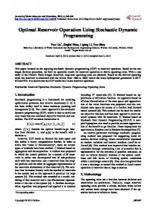
Application of FDP FDP is applied to a hypothetical reservoir system used by Larson (1968). A number of earlier methods were also applied to this system. So it is preferred to apply the present algorithm also to the same system, to make comparison of this algorithm with the earlier ones. The four dimensional reservoir network is as shown in Fig.1. Twelve time periods are considered for operating horizon, designated by 0, 1,…., 11. The constraints of four dimensional storage vector are 0 ≤ S1, t ≤10 0 ≤ S2, t ≤10 0 ≤ S3, t ≤10 0 ≤ S4, t ≤15; for t = 0,1,……,12. The constraints on release from four reservoirs are for t = 0, 1, …..,11. 0 ≤ R2, t ≤4 0 ≤ R3, t ≤4 0 ≤ R4, t≤7; 0 ≤ R1, t ≤3 th

th

where Ri, t is release from the i reservoir during time period t and Si, t is storage state of the i reservoir at beginning of time period t.

4

2

3

1

4

Figure 1: Four-reservoir system network The desired state vector at the beginning and end of operating horizon is

5 5 S0 =   5   5

S12

5  5  =  5    7 

The objective of this multireservoir system is to maximise the benefit from irrigation and hydropower generation. All the four reservoirs are used to generate hydropower. The fourth reservoir is used for both hydropower and irrigation. So the objective function is 11

4

F =∑ ∑b * R i ,t

t =0

11

i ,t

i =1

+

∑b * R 5 ,t

(4)

4, t

i =0

th

th

Where bi, t is the benefit function for i reservoir during t time period. The details of the problem are given by Larson (1968) and Heidari (1971). Depending on full range of possible inflows and possible releases from the reservoirs, maximum and minimum possible storage values are found out as given in Table 1. Table 1. Maximum/Minimum possible storage

Reservoir 1 2 3 4

0 5/5 5/5 5/5 5/5

1 7/4 8/4 9/1 12/0

2 9/3 10/3 10/0 15/0

3 10/2 10/2 10/0 15/0

4 10/1 10/1 10/0 15/0

Time steps 5 6 7 10/0 10/0 10/0 10/0 10/0 10/0 10/0 10/0 10/0 15/0 15/0 15/0

8 9/0 9/0 10/0 15/0

9 8/0 8/0 10/0 15/0

10 7/1 7/0 10/0 15/0

11 6/3 6/2 9/1 14/0

12 5/5 5/5 5/5 7/7

The corridor of five grid points with equal storage state increments at each time step is formed. The iteration continues as per the algorithm presented in the previous section. The state increments are made half continuously in each consecutive iteration. For example, the state increments during first five iterations of reservoir 2 at time step 1 are 4, 2, 1, 0.5 respectively, where as at time step 3 are 8, 4, 2, 1 th respectively. If ξ is taken as 0.002, the process converges at 5 iteration. 398.0 units is obtained as the th objective function value. If ξ is taken as 0.0004, the process converges at 7 iteration with the objective

5

function value as 398.7. This is only 0.64% less than global optimum value, which is 401.3, obtained by earlier methods. The objective function value and rate of convergence are shown in Fig. 2. The development of trajectories in alternative iterations, i.e., 1, 3, 5, are shown in Fig. 3.

400 397.2

398.7

398.6

398

396 394.4 392

391.8 .

388 385.6 384 1

2

3

4

5

6

7

8

Figure 2. Objective function value at different iterations. Naming of the Algorithm, FDP If a flexible thread is folded twice, five folding points are obtained. These five points are as five storage states in first iteration. Length between two consecutive folding points is as state increment. Taking any consecutive three points, if the thread is again folded twice, there will be two more points making up to a total of five. Now the length between two consecutive points is half of that of first folding. By repeated folding like this, we can reach to any point of the whole of the thread. Authors visualized the importance of folding phenomenon to reach to any value of feasible storage from whole range of storage state. Hence the name is given as folded DP. Conclusions A new algorithm to over come the curse of dimensionality problem in dynamic programmig is presented and applied to a hypothetical multi reservoir system. In the earlier methods, an initial feasible trial trajectory is essential to start. The trial trajectory moves towards the global optima in the grid of state increments. Trajectory may fall into local optima, if it is in between initial trial trajectory and global one. To over come this problem, Bellman has suggested solving the problem with different trial trajectories. But if the dimension, i.e., number of reservoirs in the system, is large, there is no clue as to the number of trial trajectories required to ensure the global optimum condition. The above inconvenience could be avoided in present algorithm, as no initial trajectory is necessary. In earlier algorithms, the convergence depends on the distance between initial trial trajectory and the optimal trajectory. But in the present method, there is no such depending factor for convergence. From the algorithm, it can be seen that the present method takes remarkably less iterations than earlier methods to converge. The rate of improvement slows down at higher number of iterations, which can be seen in Fig. 2 and Fig. 3. The only disadvantage in the present algorithm is that there is no guarantee of reaching at the global optimum which is the case with most of the earlier methods. Heidari et al. (1971) have agreed in their paper that the global optimum was found by luck, as the optimum trajectory happens to fall only on integer value and they have chosen state increment as 1.0. While solving with a state increment of 1.3, optimum objective function value was obtained as 399.06 which is less than the global optimum.

10 8 Volume)

Storage State (Unit

6

r e s e r v o ir 1

6

Ite r a tio n 1 Ite r a tio n 3 Ite r a tio n 5

4 2 0 0

2

4

6

8

10

12

10 8 Volume)

Storage State (Unit

P e r io d (t w o H o u r ly )

r e s e r v o ir 2

6 4

It e r a t io n 1 It e r a t io n 3 2 It e r a t io n 5 Fig. 3: Trajectory of the system at various iterations. 0 2

4

8 10 FF 6 P e r io d (T w o H o u r ly )

12

10 r e s e r v o ir

8 Volume)

Storage State (Unit

0

3

Ite r a tio n 1 Ite r a tio n 3 Ite r a tio n 5

6 4 2 0 0

2

4

6

8

10

12

Volume)

Storage State (Unit

P e r io d ( T w o H o u r ly )

14 12 10 8 6 4 2 0

r e s e r v o ir 4 It e r a t io n 1 It e r a t io n 3 It e r a t io n 5

0

2

4

6

8

10

12

P e r io d (T w o H o u r ly ) Figure 3. Trajectory of the system at various iterations a. Reservoir 1, b. Reservoir 2, c. Reservoir 3, d. Reservoir 4

7

M

M

The required matrix size in the present algorithm is number of time periods * 5 * 5 instead of number of M M time periods * 3 * 3 as in the case of IDP. So in the application of FDP, the required matrix size is 12 * 625 * 625. In case of multireservoir system, the matrix size increases exponentially. In this situation, FDP can be applied with successive approximation, i.e. considering only one dimension at a time. So the matrix size in each iteration will be number of time periods * 5 *5. It is concluded that FDP can be used as an improvement to IDP. In case of higher dimensional problem, FDP can be solved in successive approximation. References Bellman, R., Dynamic programming, Princeton University Press, Princeton, N. J., 1957. Falguni Baliarsingh (2000). “Long-term and short-term optimal reservoir operation for flood control”, Ph.D. thesis, Indian Institute of Technology, Kharagpur, India. Giles, J. E., and Wunderlich, W. O. (1981). “Weekly multipurpose planning model for TVA reservoir system.” J. Water Resour. Plng. and Mgmt., ASCE, 107(WR2), 495-511. Hall, W. A., Tauxe, G. W., and Yeh, W. W-G. (1969). “An alternate procedure for the optimization of operations for planning with multiple river, multiple purpose systems.” Water Resour. Res., 5(6), 13671372. Heidari, M., Chow, V. T., Kokotovic, P. V., and Meredith, D. D. (1971). “Discrete differential dynamic programming approach to water resources systems optimization.” Water Resour. Res., 7(2), 273-282. Larson, R. E., and Korsak, A. J. (1970). “A dynamic programming successive approximations technique with convergence proofs.” Automatica, 6, 245-252. Ozden, M. (1984). “A Binary State DP algorithm for operation problems of multireservoir systems.” Water Resour. Res., 20(1), 9-14. Perera, B. J. C., and Codner, G. P. (1998). “Computational improvement for stochastic dynamic programming models of urban water supply reservoirs.” J. American Water Resour. Assoc., 34(2), 267278. Trott, W. J., and Yeh, W. W-G. (1973). “Optimization of multiple reservoir system.” J. Hydrol., 99(HY10), 1865-1884. Turgeon, A. (1981). “Optimal short-term hydro scheduling from the principle of progressive optimality.” Water Resour. Res., 17(3), 481-486. Yakowitz, S. (1982). “Dynamic programming applications in water resources.” Water Resour. Res., 18(4), 673-696. Yeh, W. W-G. (1985). “Reservoir management and operations models a state-of-the-art review.” Water Resour. Res., 21(12), 1797-1818.