Formulae for Computing Logarithmic Integral Function ( )=∫ Amrik Singh Nimbran 6, Polo Road, Patna, INDIA Email:
[email protected] Abstract: The prime number theorem states that the number of primes up to a given number is approximated by the logarithmic integral function. To compute the value of this function, the author offers two formulae deduced from truncated series – one convergent and the other divergent. He also gives a table of values computed by him for this function. Key words: Prime numbers, prime counting function, logarithmic integral function. AMS Classification: 11A41, 26A Introduction: Hadamard and de la Vallée Poussin independently showed in 1896 that if π( ) denotes the number of primes up to a given number , then for some positive constant √
π( ) = Li( ) + O(
).
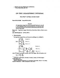
Here Li( ) = ∫
is the logarithmic integral function. Some books on number
theory record the values of Li( ) for certain without giving any clue to the method by which these values have been arrived at. We find the following expansion at some places [1]: (
Li( ) = ∑
)!
+O
(1)
In this paper, I offer two alternative series for computing Li( ). Let us take the identity:
= + 1+ + !
!
+ + !
!
+⋯
!
+⋯
(2)
Term-by-term integration of the right hand side and repeated integration ‘by parts’ of the left hand side lead to: RHS = ln + LHS =
+
+ +
. !
!
+
. !
+… +
+ ⋯ +
Putting u = ln , du =
(
)!
,
. !
+⋯
(3)
+⋯
(4)
= t, we obtain from (2), (3) and (4): 1
∫
= ln ln + ln +
∫
=
+
!
+
. !
+
. ! !
+
+ ⋯ +
+ ⋯ +
. ! (
+⋯
)!
(5)
+⋯
Now taking the definite integral: Li( ) = ∫
(6) , we obtain two alternative expansions
– while (5) gives a convergent series, (6) results in a difference of two divergent series. I have found on close examination that we may usefully employ truncated versions of these expansions for computing Li( ). Let me first introduce two theorems which analyse the behaviour of the terms in (5) and (6). Theorem 1:
=
. !
attains the maximum value at
= [ln ] − 1 or at
= [ln ] − 2 for
= [ln ] − 1 for
≥ 91, this will
≥ 91.
all
Proof: If we show that < and suffice. Now [ln ] = (ln ) − , 0≤
at
}
)
}
and for denominator to be non-zero and positive, it is necessary that ln ln ≥ 4, i.e., ≥ 55.
>
+ 3, i.e.,
Now numerator − denominator =( + 2) − ( + 1) ln . Thus
(
)
(
)
< ln which implies that
< 1, i.e., if ln ≥ , or
≥ 91,
. We have thus shown that for Thus either = [ln ] − 1 or at
− (1 − ), ln > 0 as
≥ 91 and
= [ln ] − 1,
+ 1, i.e.,
< 1. Hence for
.
or is the largest term, i.e., attains the maximum value at = [ln ] − 2 for ≥ 91. Generally, it is at = [ln ] − 1 that =10
2
attains the maximum value but occasionally as is the case for = [ln ] − 2. ⧠
=3 and
=10, it may be at
It is thus clear that the terms in (5) first increase, attain the maximum value and then begin decreasing to approach zero. Theorem 2:
=
(
)!
attains the minimum value at = [ln ] + 1, where [ln ] denotes the
greatest integer contained in ln . Proof:
=
;
=
Putting n=[ln ] +1, ≤
i.e.,
=