Proceedings of the International MultiConference of Engineers and Computer Scientists 2008 Vol I IMECS 2008, 19-21 March, 2008, Hong Kong
Foundations of Interval Computation Trong Wu Abstract. This paper reports a study of numerical computation problems from a theoretical viewpoint. It shows that computer systems are not capable of computing of real numbers correctly due to the differences between the algebraic structures of real numbers and model numbers. These two classes of numbers are not isomorphic. From this study, we have learned that there are no machine errors or computation errors. If fact, one can view it is a human mistake by putting real valued problem onto a model number platform for computation. This paper proposes use of the concept of computer model numbers to approximate rough numbers for computation. Moreover, we revise an arbitrary initial compact interval to a shortest initial closed-open model interval for ordinary interval computation. This way, we can assure that the final resulting interval will be the shortest interval and that the computation will result in the greatest precision. Index terms: Interval Arithmetic, Algebraic Structures, Isomorphic, Model Numbers, Dyadic Numbers
I. INTRODUCTION In 1982, Pawlak proposed a concept called rough sets, used in the theory of knowledge for the classification of features of objects [Pawlak1982]. He considered X to be a set and R to be a relation over X. The pair (X, R) is called a rough space, and R is called the rough relation. If xRy, then one could say that x is too close to y, x and y are indiscernible, and x and y belong to the same elementary set. The concept of rough sets is usually used in knowledge representation. Later, Wu [1994, 1998] defined a new class of real numbers called rough numbers, the definition is given in Section 4, which is a one-dimensional rough set in rough set theory. Most computer users are not aware the computation of real numbers and rough numbers are not the same. Some programming languages, such as FORTRAN, COBOL, Pascal, etc., create more confusion by allowing programmers to declare variables with type real in their programs for computations. To fully understand the problems of real number computation with computers, we must study the algebraic structures for the set of all real numbers and the set of all rough numbers over computer systems. This not only provides the theoretical foundation for computer arithmetic, but also interprets rounding errors, machine errors, and computation errors from algebraic structure viewpoint. In this paper, we revise ordinary interval computation, given by Moore [1966] from a short
ISBN: 978-988-98671-8-8
compact interval [a, b] of real numbers a and b for a given real number r, where a = r − δ, b = r + δ, and δ is an arbitrary small number, to the shortest closed-open interval [a, b) with exactly represented by computer numbers, a and b for all initial intervals in computation. To implement this, we consider for each real number x within the computer range; let a be the downward rounding value of x, let s be the smallest positive number, with respect to x, such that a + s > a, and let b = a + s. Thus [a, b) is the shortest closedopen interval for x on the given computer system, where a and b are the numbers that the computer system can represent them exactly. This new method will provide the shortest resulting interval. To study the computation of real numbers, it is important to begin by studying the structure of rough numbers with respect to a given computer system. The difficulty of numerical computation [Aberth 1988, Wu 1993] within computer systems is that one must work with two distinct number systems. Specially, solving any numerical computation problem consists of the following three parts. (1) The problem is given in the real number system. (2) The computation is done in the model number (an Ada language terminology, see Section 4 for definition) system of the given machine, M. (3) The results must be converted from model numbers into real numbers. These two number systems have different algebraic structures, and they are not isomorphic. Therefore, a problem moving from platform (1) to platform (2) for computation can induce incorrect results and so can moving from platform (2) to platform (3). The platform (2) can only provide an approximated result for platform (1); these incorrect results do not contain machine errors and computation errors because the computer system performances exactly work as requested. Therefore, it has no rounding errors. In fact, one can view this a human mistake by putting a real valued problem onto a model number platform for computation. Since the difference between correct results and incorrect results are not known, thus applying the results of a computation to a science or engineering application is an un-decidable problem. For this reason, an interval computation is applied so that it will make this un-decidable problem becomes a decidable problem [Moore 1966]. Moreover, this paper will show that revised interval computation can assure that the final resulting interval will represent a shortest interval. According to the author’s best knowledge there is lacking of the study of number structures for numerical computation in the record of literatures. It took author more then ten years to develop the foundation of this paper since
IMECS 2008
Proceedings of the International MultiConference of Engineers and Computer Scientists 2008 Vol I IMECS 2008, 19-21 March, 2008, Hong Kong
last two papers [Wu, 1994 and 1998] were presented at conferences. Now, we can introduce some basic algebraic structures, the structures of dyadic numbers and rough numbers. Then we will consider rough numbers for interval computation.
II. SOME BASIC ALGEBRAIC STRUCTURES OF NUMBERS For solving a numerical computation problem, there exists a fundamental crisis in the algebraic structure of numbers. Different classes of numbers have different algebraic structures. Therefore, we must study some basic algebraic structures of numbers. In fact, the algebraic structures of real numbers, dyadic numbers, and rough numbers are all different. We will begin with the definition of an abelian group, then extend it to include a ring and a field [Waerden 1948, Herstein 1971]: Definition 2.1 An abelian group (G; +) is a set G together with a binary operation namely, addition, “+”,which satisfies the following conditions [Waerden 1948, Herstein 1971]: (1) For all a, b ∈ G, such that a + b ∈ G. (2) For all a, b, c ∈ G, then (a + b) + c = a + (b + c). (3)There is an identity element, e in G such that a + e = e + a, for all a ∈ G. (4) For all a ∈ G, there exists an inverse, (−a), such that (−a) + a = a + (−a) = e. (5) For all a, b ∈ G, such that a + b = b + a. Example 2.1 The set of all integers, I, with usual addition, +, (I, +), is an abelian group. A ring structure is a special case of an abelian group. By adding two additional conditions to an abelian group, it forms a ring [Waerden 1948, Herstein 1971]: Definition 2.2 We say that (S; +, ×) is a ring, if (S; +) is an abelian group, defining × as a mapping from S × S → S, which satisfying the following conditions: (1) For all a, b, c ∈ S, then (a × b) × c = a × (b × c). (2) Multiplication is distributed over addition: that is for all a, b, c ∈ S, the left and right distributive laws hold: a × (b + c) = a × b + a × c, and (b + c) × a = b × a + b × c. Example 2.2 The set of all integers I with usual addition, +, and multiplication, × , then (I, +, ×) is a ring. This ring has no zero-divisor. A field is a commutative ring accompanied by unity with respect to multiplication and every non-zero element has a multiplicative inverse [Waerden 1948, Herstein 1971]. Definition 2.3 A Field (F; +, ×) is a ring with commutative law and multiplicative unity such that each
ISBN: 978-988-98671-8-8
non-zero element has a multiplicative inverse that satisfies the following conditions: (1) For all a, b ∈ F such that a × b = b × a. (2) There exists 1 such that a × 1 = 1 × a = a. (3) For each non-zero element a in F there is an inverse (1/a) such that a × (1/a) = (1/a) × a = 1. Example 2.3 The set of all rational numbers, real numbers, and complex numbers with usual addition, +, and multiplication, ×, are fields. Let F be a field, the set of all polynomials in the indeterminate, x, with coefficients in F and written as F[x], then following theorem (without proof) determines a ring of polynomials [Waerden 1948, Herstein 1971]: Theorem 2.1 Let F be a field, the set of all polynomials a0 + a1x + a2x2 + …+ anxn, written as F[x], where n can be any non-negative integer and ai (i = 0, 1, …, n) are all in F. Then F[x] is a ring under the operation induced by the operations in F. It is known that the set of all real numbers, denoted E, together with arithmetic, addition, + and multiplication, × forms a field. Human arithmetic, such as + and ×, always returns exact results. On the other hand, most computer systems can store only certain real numbers exactly in the memory. Some of these real numbers are 100.5, 70.875, 12.375, 0.5, 87.125, etc. Some other real numbers such as 0.1, 0.2, 0.3, 0.4, 0.6, etc. have a binary representation with infinitely many digits; they cannot be stored in the memory exactly. This tells us that a computer system cannot represent these real numbers. Therefore, the set of all numbers represented by the computer for computation with the usual addition, +, and multiplication, ×, operations are not the same as the set of all real numbers. Even if we allow a computer system to have as many bits as required to store a floating-point number, it still is not able to contain the multiplicative inverse for all numbers in the computer system. This is because these computer numbers do not form a field. It is a subset of a ring with ring operations. The structures of the set of all real numbers and the set of all the numbers in the computer system are quite different. No one-to-one correspondence onto function f from the set of real numbers to the set of all computer numbers exists. The set of all computer numbers is known as model numbers in the Ada programming language [Barnes 1989, 1992, 1995, Watt et al. 1987]. Moreover, f does not preserve the algebraic structure of real numbers and f cannot be a local homomorphism between the set of real numbers within a given range of machine M and the set of all computer numbers; they are not isomorphic. This leads to a computation of + and × over the set of all model numbers represented by a computer system that produce an incorrect result for the given problem. Therefore, computer users should know that the current Von Neumann architecture computer systems could only provide some approximations for numerical computation. Next, we will need to find out the actual structure of computer-
IMECS 2008
Proceedings of the International MultiConference of Engineers and Computer Scientists 2008 Vol I IMECS 2008, 19-21 March, 2008, Hong Kong
represented numbers. In other words, what kind of arithmetic can computer systems do? So, we turn to study the set of dyadic numbers [Kelley 1955].
III. THE STRUCTURE OF DYADIC NUMBERS We require that for each non-negative real number x can have its b-adic expansion, where b is an integer greater than 1. Actually, we want to write a real number x as the sum of multiples of powers of b, where the multiples are non-negative integers less than b. Clearly, the b-adic expansion of the number may fail to be unique in a decimal expansion, .9999. . . (all nines) and 1.0000 . . . (all zeros) are to be expansions of the same real number. When b = 2, the b-adic expansions are then called dyadic expansions and numbers written as dyadic expansions are called dyadic numbers [Kelley 1955]. Theorem 3.1 For each real number x and B ={0, 1}, we have its dyadic expansion over a finite field (B; +, ×): ∞
x = sign
∑a 2
{
}
, where ai ∈ B and sign ∈ + ,− .
i
i
(3.1)
i =−∞
A computer system is a finite state machine; therefore, it is capable of representing only a finite set of numbers internally. Thus, any attempt to use a digital computer to do arithmetic in the set of all real numbers is doomed to failure. The set of all real numbers is an infinite set and most of the elements in the set cannot be represented by a computer system. Therefore, for theoretical reasons, we may assume that a computer system can have any finite number of bits to store its numbers, integers and floatingpoint numbers. For any non-negative integer n, we consider the set of all numbers with the representation: n
y = sign
∑a 2 i
i
{
}
, where ai ∈ B and sign ∈ + ,− . (3.2)
i =− n
This representation contains two parts, one is with index 0 ≤ i ≤ n and the other is with an index −1 ≤ i ≤ −n. The former is the integer part of y and the latter is the fraction part of y, respectively. In this paper, we will define a structure for the set of all numbers with this representation and it is called the set of all finite (term) dyadic numbers, FD, and the term finite means any finite value: FD =
{
n
y | y = sign
∑a 2 i
i =− n
i
{
}
, ai ∈ B, sign ∈ + ,−
}
and n is a non-negative integer .
(3.3)
From Definitions 2.2, 2.3, and 2.4, we see that all finite (term) dyadic numbers comprise neither a ring nor a field. Moreover, it is a subset of ring of polynomials of 2 over a finite field B = ({0, 1}; +, ×). In fact, each computer system can have only a fixed number of bits of memory space to store a number of its type such as integer, float, double, . . ., etc. An integer
ISBN: 978-988-98671-8-8
within the computer-predefined range often can be represented exactly. However, a real number within the range usually cannot be represented correctly. Today, most computer systems implement the IEEE 754 floating-point number format [IEEE1985] for storing real numbers. For example, a 32-bit floating-point number format is divided into four areas: a sign bit sign, an 8-bit exponent Exp, a hidden bit, and a 23-bit mantissa M: sign × (1.M) × 2Exp-127,
(3.4)
where sign = ‘0’ indicates a positive value, sign = ‘1’ indicates a negative value. The 1 in (1.M) is the hidden bit, the M is a 23-bit mantissa, and the exponent Exp is an unsigned integer in {0, 1, 2, … 255}. It is clear that a floating-point number represented in (3.4) is a special case of a limited dyadic number with limited number of n which is a finite (term) dyadic number given in the set of FD in (3.3). Again, computer systems can only use a limited number of bits to represent a floating-number. Therefore, ring computation, such as + and ×, can cause an overflow or underflow. Most computer systems use floating-point number arithmetic for numerical computation, and most computer users are not aware that floating-point number arithmetic often produces a different result from the truly correct result in real numbers. This is not avoidable. In general, the output of a numerical computation program from one machine can be different from the output from another machine.
IV. THE STRUCTURE OF ROUGH NUMBERS The Ada programming language [Watt 1987] calls a real number a model number, if the real number can be stored exactly in a computer system with a radix of power of 2. Therefore, the set of all model numbers is a subset of dyadic numbers and we call it the set of limited dyadic numbers with respect to a given computer system. The term limited reflects the given computer system’s word size for floating-point numbers. For those real numbers that cannot be stored exactly in a given computer system, we call them rough numbers with respect to the given computer system. In order to study this large class of numbers, it is necessary to define rough numbers precisely and mathematically. Definition 4.1 Let E be the set of all real numbers within the range of a given computer system M, and let R be a relation on E. The pair (E, R) is called rough space and R is called the rough relation, if x, y ∈ E and (x, y) ∈ R, we say that x and y are indistinctive in the rough space (E, R) with respect to the given computer system M. We call x and y rough numbers and they are approximated to the same model number. If a real number is a model number with respect to a given machine M, then it is a special case rough number. Most computer systems use a downward rounding policy to approximate a rough number with a model number. Thus, there are infinitely many rough
IMECS 2008
Proceedings of the International MultiConference of Engineers and Computer Scientists 2008 Vol I IMECS 2008, 19-21 March, 2008, Hong Kong
numbers approximated by the same model number, such that all rough numbers z ∈ [x, y) are approximated by the same value of the model number x for computation [Wu 1994, 1998]. Throughout this paper, we will also use a downward rounding policy to handle the approximation of rough numbers. Theorem 4.1 Let E be the set of all real numbers within the range of a given computer system M, and let R be a relation on E. If x, y ∈ E and (x, y) ∈ R in the rough space (E, R) then R is an equivalence relation on E. (Readers may verify this theorem) Equivalence classes of the relation R are called basic model intervals [Watt et al. 1987, Ada 9X Mapping/Revision Team 1993], the smallest interval with model number endpoints. The set of all basic model intervals in (E, R) is denoted by E/R. The definition of a rough number is a special case of the one-dimensional rough sets given by Pawlak [Pawlak 1982]. In reality, for any rough number z whose value is within the range of a given computer system M, there exists a smallest closedopen interval, such that
⎡ ⎣
z∈ ⎢i +
k −1 k ⎞ ,i + n ⎟ , n 2 2 ⎠
(4.1)
for some positive integers n and k. where the lower bound is the approximation of z, i is the integer part of z, k is an integer with 0 ≤ k ≤ 2n − 1, and n = n(be, bm), a function of the number of bits in the field of exponential be and the number of bits in the field of mantissa bm. The difference between the rough number z, and its approximation given in (4.1) is given by (4.2):
⎛ ⎝
z − ⎜i +
k − 1⎞ ⎟. 2n ⎠
(5.1) f(a + b) ≠ f(a) ⊕ f(b) They are two different additions. In the inequality (5.1), computations occur over two different number systems; we need to adjust by adding an error term, Err, to form the equality: f(a + b) = f(a) ⊕ f(b) + Err. (5.2) This error term, Err, commonly is called rounding-error.
Real numbers
Dyadic numbers
(A field)
ab a +b
f ⎯ ⎯ →
f (a +b) f (a) ⊕ f (b)
(4.2)
This is also called rounding-error. Usually, a programmer is either unaware of the existence of rounding-errors or unable to reduce or control them in the course of a computation. In fact, every real number is a rough number from computer system viewpoint. We will see that the set of all rough numbers over the set of all computer systems has the dyadic number structure.
V. HIERARCHICAL CLASSES AND COMPUTATION In mathematics, we have learned the properties of several classes of numbers such as integers, rational numbers, irrational numbers, and real numbers. However, a computer system can have only a limited word size; therefore, only some integers and some rational numbers can be computed correctly in a computer system. Other numbers cannot even be represented exactly in a computer system.
ISBN: 978-988-98671-8-8
Computer systems handle real numbers in a binary fashion. For each real number x, we have its dyadic expansion over the finite field (B; +, ×). Among all the dyadic numbers, only a limited number of dyadic numbers can be computed in a computer system. The relationship of the set of real numbers and the hierarchical structures of dyadic numbers is shown in Figure 5.1. The set of real numbers has a field structure, while the set of finite dyadic numbers is not a field; it is a subset of ring. f is not a one-to-one and onto function, f does not preserve the field structure, and cannot even be a local homomorphism between the set of real numbers within a given range of machine M and the set of limited dyadic numbers. The addition ‘+’ on the left hand side of the inequality (5.1) is a field addition and the addition ‘⊕’ on the right hand side is a ring addition over dyadic numbers.
Rough numbers
Finite dyadic numbers Limited dyadic numbers (model numbers)
(A subset of a polynomial ring) Figure. 5.1 Hierarchical structures of dyadic numbers Unfortunately, most programming textbooks do not teach students the addition ‘+’ in a program is not real number addition, but a dyadic number addition instead. Many computer users are misled and disappointed that computer systems cannot provide accurate results for computations. From the theoretical viewpoint, a computer system cannot compute real numbers correctly. Therefore, applying the results of computation to a real world problem is an un-decidable problem. We introduce a different
IMECS 2008
Proceedings of the International MultiConference of Engineers and Computer Scientists 2008 Vol I IMECS 2008, 19-21 March, 2008, Hong Kong
method of computation called interval computation [Moore 1966, 1979, Alefeld et al. 1983] that will provide a shortest interval for the result; it gives the result in an interval, the length of the interval provides the maximum error for computation, this way it will turn the problem into a decidable problem. To implement interval computation we will need a special programming language. Among all commonly used programming languages, the Ada programming language is a unique language that allows the user to define a specific model number for their rough numbers for dealing with computation. In the next section, we will suggest a new computational method for the set of all rough numbers called model interval computation that can provide verification of the magnitude of the absolute error.
VI. A MODEL INTERVAL COMPUTATION For any real numbers x and y, there exist basic model intervals X = [a1, b1] and Y= [a2, b2] such that x∈ [a1, b1) and y∈[a2, b2) where a1, b1, a2, and b2 are model numbers. For a real number z that is a model number, we consider a special case Z = [z, z1], where z1 is the smallest model number greater than z. Then, the usual computer scalar arithmetic operations, addition +, subtraction −, multiplication ×, and division /, are defined for interval computation. Therefore, the sum, difference, product, and quotient of two real numbers are all within a given interval respectively. We use revised closed-open intervals to exclude the upper endpoint for interval computation. The results are shown here: Addition x + y ∈ [[a1, b1] + [a2, b2] ) = [a1 + a2,, b1 + b2). (6.1) Subtraction x − y ∈ [[a1, b1] − [a2, b2] ) = [a1 − b2,, b1− a2). Multiplication x × y ∈[ min(a1a2, a1b2, b1a2, b1b2), max(a1a2, a1b2, b1a2, b1b2)). Division
(6.2)
(6.3)
1/y ∈ [1/b2, 1/a2), if 0 ∉ B, then we define x/y ∈ [min(a1/b2, a1/a2, b1/b2, b1/a2), max(a1/b2, a1/a2, b1/b2, b1/a2))
(6.4)
The deficiency of interval arithmetic is the use of real numbers for the lower bound and upper bound for the interval. In general, a real number cannot be represented exactly by the floating-point number format. A better way to perform interval computation and reduce rounding-error is (1) to create the smallest closed interval, containing the given real number, with model numbers for the lower and upper bounds, and (2) to develop bit-to-bit computation over the mantissa, the internal representation of model numbers.
ISBN: 978-988-98671-8-8
Since the product of two model numbers or the inverse of a model number might not be a model number, we round the result outward to the nearest model numbers. Let m(x) be the greatest model number less than x for the lower bound and m(y) be the smallest model number greater than y for the upper bound. Therefore, we redefine multiplication and division as follows: Multiplication x × y ∈[m(min(a1a2, a1b2, b1a2, b1b2)), (6.3)’ m(max(a1a2, a1b2, b1a2, b1b2))). Division 1/y ∈ [1/b2, 1/a2), if 0 ∉ B, then we define x/y ∈ [m(min(a1/b2, a1/a2, b1/b2, b1/a2)), (6.4)’ m(max(a1/b2, a1/a2, b1/b2, b1/a2))). Moore [1966] proved an important theorem that supports interval computation and since then interval computation has become a new and growing branch of applied mathematics. We call this theorem the fundamental theorem of interval computation. It is necessary to quote the theorem here to support our work. Theorem 6.1 The Fundamental Theorem of Interval Computation: Let f(x1, x2, . . . , xn) be a rational function of n variables. Consider any sequence of arithmetic steps which serve to evaluate f with given arguments x1, x2, . . . , xn. Suppose we replace the arguments xi by the corresponding closed interval Xi (i = 1, 2, . . . , n) and replace the arithmetic steps in the sequence used to evaluate f by the corresponding interval arithmetic steps. The result will be an interval f(X1, X2, . . . , Xn). This interval contains the value of f(x1, x2, . . . , xn), for all xi ∈ Xi (i= 1, 2, . . . , n). Later, Moore [1979] and Alefeld and Herzberger [1983] gave some algebraic properties of interval arithmetic. From Figure 5.1, let RD be the set of all rough numbers or dyadic numbers, FD be the set of all finite dyadic numbers, and LD be the set of all limited dyadic numbers or model numbers with respect to a given machine M, then we have the following set hierarchical structures: LD ⊂ FD ⊂ RD. (6.5) By definition, we see that every real number is a rough number from computer system viewpoint. In fact, the computation is done in the set of LD, and computation of any rough numbers outside the set LD and within the range of a given machines M would round down to a model number in the set of LD for computation. This would generate a rounding-error. In the model interval computation, any rough numbers outside the set LD and within the range of a given machines, M would round down to a shortest model interval in the set of LD for computation. This would minimize the resulting interval for the computation.
IMECS 2008
Proceedings of the International MultiConference of Engineers and Computer Scientists 2008 Vol I IMECS 2008, 19-21 March, 2008, Hong Kong
VII. CONCLUSION In this paper, we have reviewed some basic algebraic structures such as abelian groups, rings, and fields. We defined sets of rough numbers, dyadic numbers, finite dyadic numbers, limited dyadic numbers, and model numbers; from these definitions, we have learned that the difficulty of numerical computation is that one must actually work with two distinct number systems. Solving any numerical computation problem consists of the following three parts: (1) the problem is given in the real number system, (2) the computation is done in the model number system for the given machine, and (3) the results must be converted from model numbers into real numbers. Real numbers and model numbers have two different algebraic structures, and they are not isomorphic. In general, starting from the problem to computation on a machine often generates incorrect results and going from the machine computation to reporting results in real numbers can have incorrect results too. This paper has reported that a computer system is not capable of computing real numbers accurately within its constraints from algebraic structure viewpoint. Computation over the set of real numbers requires performing a field computation. However, when a real number within the given range is stored or read into a computer system, it is converted into a dyadic number. Computation over the set of limited dyadic numbers is dyadic number computation. If f be a mapping that takes each real number into its dyadic number representation; it is not a one-to-one and onto function. If a and b are two real numbers within a given range and they map into their dyadic representations f(a) and f(b), respectively, then in general, we should have f(a + b) ≠ f(a) + f(b). The addition, +, is the addition of real numbers. The mapping f does not preserve the algebraic structure, so the set of real numbers and the set of dyadic numbers are not isomorphic. To avoid overloading and possible confusion, we will introduce a new addition ‘⊕’ for the dyadic number addition. To adjust the inequality, we will add in an error term, Err. Therefore, we have f(a + b) = f(a) ⊕ f(b) + Err. In addition, we have revised interval arithmetic from real number ending points to model numbers and from a closed interval to a closed-open interval. This will eliminate possible rounding errors, perform a bit-to-bit computation, create the shortest initial intervals for each initial real number, and ensure the resulting interval is the shortest one in the given machine. In this paper, we have successfully redefined overloading for +, −, ×, and / on internal binary representations so that we can create the lower bound and the upper bound in model numbers for a given real number. Also, we have carefully developed bitto-bit model interval computation [DEC 1985, IBM 1992]. For each initial real number, we have created the shortest model interval to include the real number for computation with the required precision. This is a very important step
ISBN: 978-988-98671-8-8
because only with the shortest initial intervals can one obtain the maximum precision form the given machine. This model interval computation not only provides an approximation for the solution but also gives the length of the resulting interval that is the maximum possible of error due to human mistake. Therefore, it can be used for any numerical computation problem, in particular, for any accuracy critical problems. ________________________________________________ The Author: Trong Wu is a Professor in the Department of Computer Science, at Southern Illinois University Edwardsville, Edwardsville, Illinois 62026 U.S.A. e-mail:
[email protected]; Phone: 618-650-2393.
REFERENCES Aberth, O., 1988. Precise Numerical Analysis, Dubuque: Wm C Brown Publishers. Ada 9X Mapping/Revision Team, 1993. .Ada 9X Rationale, Intermetrics Inc. Cambridge, Mass. Alefeld, G. and Herzberger, J., 1983. Introduction to Interval Computations, New York: Academic Press, Barnes, J. G. P., 1989. Programming in Ada, 3rd Ed., AddisonWesley Publishing, Reading Massachusetts. Barnes, J. G. P., 1992. Programming Language in Ada, 4th Ed. Addison-Wesley Publishing Company. Barnes, J., 1995. Programming in Ada 95, Addison-Wesley Publishing, Reading Massachusetts. DEC, 1985. Vax Ada Language Reference Manual, Digital Equipment Corporation, Maynard, Mass. Herstein, I. N., 1971. Topics in Algebra, University of Chicago. IBM (AIX), 1992. Ada/6000 User's Guide, IBM Canada Ltd. Laboratory, North York, Ontario, Canada, M3C 1W3. IEEE Inc., 1985. IEEE Standard for Binary Floating-point Arithmetic (ANSI/IEEE std 754-1985), New York Kelley, J. L., 1955. General Topology, D. Van Nostrand Company, Inc. Moore, R. E., 1966. Interval Analysis, Prentice-Hall, Englewood Cliffs, New Jersey. Moore, R. E., 1979. Methods and Applications of Interval Analysis: SIAM Studies in Applied Mathematics, 2, Philadephia: Society for Industrial and Applied Mathematics. Pawlak, Z., 1982. Rough Sets, International Journal of Computer and Information Sciences, V. 11, No. 5, 341-356. Waerden, V. D., 1948. Modern Algebra, English edition, Julius Springer, Berlin. Watt, D. A., 1987. Wichmann, B. A., and Findlay, W., Ada Language and Methodology, Prentice-Hall, Englewood Cliffs, New Jersey. Wu, T., 1993.An Accurate Computation of the Hypergeometric Distribution Function, ACM Transactions on Mathematical Software, V.19, No. 1, 33-43. Wu, T., 1994. Rough Number Structure and Computation, Proceedings of the Third International Workshop on Rough Sets and Soft Computing, 360-367.
Wu, T., 1998. Rough Numbers and Computations, 1998 IEEE World Congress on Computational Intelligence Proceedings Fuzz-IEEE’98, 845-890.
IMECS 2008