Foundations of recommender system for STN localization during DBS surgery in Parkinson’s patients Konrad Ciecierski1 , Zbigniew W. Ra´s2,1 , and Andrzej W. Przybyszewski3 1
Warsaw Univ. of Technology, Institute of Comp. Science, 00-655 Warsaw, Poland Univ. of North Carolina, Dept. of Comp. Science, Charlotte, NC 28223, USA 3 UMass Medical School, Dept. of Neurology, Worcester, MA 01655, USA
[email protected],
[email protected],
[email protected]
2
Abstract. During deep brain stimulation (DBS) treatment of Parkinson disease, the target of the surgery is the subthalamic nucleus (ST N ). As ST N is small (9 x 7 x 4 mm) and poorly visible in CT4 or MRI5 , multi-electrode micro recording systems are used during DBS surgery for its better localization. This paper presents five different analytical methods, that can be used to construct an autonomic system assisting neurosurgeons in precise localization of the ST N nucleus. Such system could be used during surgery in the environment of the operation theater. Signals recorded from the micro electrodes are taken as input in all five described methods. Their result in turn allows to tell which one from the recorded signals comes from the ST N . First method utilizes root mean square of recorded signals. Second takes into account amplitude of the background noise present in the recorded signal. 3rd and 4th methods examine Low Frequency Background (LF B) and High Frequency Background (HF B). Finally, last one looks at correlation between recordings taken by different electrodes. Keywords: Parkinson’s disease, DBS, STN, FFT, DWT, RMS, LFB, HFB, Hierarchical clustering
Introduction Parkinson disease (PD) is chronic and advancing movement disorder. The risk factor of the disease increases with the age. As the average human life span elongates also the number of people affected with PD steadily increases. PD is primary related to lack of the dopamine, that after several years causes not 4 5
Computer Tomography Magnetic Resonance Imaging
2
Konrad Ciecierski, Zbigniew W. Ra´s, Andrzej W. Przybyszewski
only movement impairments but also often non-motor symptoms like depressions, mood disorder or cognitive decline therefore it has a very high social cost. People as early as in their 40s, otherwise fully functional are seriously disabled and require continuous additional external support. The main treatment for the disease is pharmacological one. Unfortunately, in many cases the effectiveness of the treatment decreases with time and some other patients do not tolerate anti PD drugs well. In such cases, patients can be qualified for the surgical treatment of the PD disease. This kind of surgery is called DBS6 . Goal of the surgery is the placement of the permanent stimulating electrode into the ST N nucleus. This nucleus is a small – deep in brain placed – structure that does not show well in CT or MRI scans. Having only an approximate location of the ST N , during DBS surgery a set of parallel micro electrodes are inserted into patient’s brain. As they advance, the activity of surrounding neural tissue is recorded. Localization of the ST N is possible because it has distinct physiology and yields specific micro electrode recordings. It still however requires an experienced neurologist / neurosurgeon to tell whether recorded signal comes from the ST N or not [3]. That is why it is so important to provide some objective and human independent way to classify recorded signals. Analytical methods described in this paper have been devised with exactly that purpose. Taking as input recordings made by set of electrodes at subsequent depths they provide information as to which of the electrodes and at which depth passed through the ST N .
1
Signal filtering
Wavelet transforms do not assume stationarity of the signal. It comes from the fact that wavelet base function is also time localized - not stationary. Because of this, the information regarding time in which certain frequencies are present is preserved. From this, looking at specific wavelet transform one can easily identify corresponding sample ranges in raw unfiltered signal [1]. In the case of DWT7 there are many functions that can be used as a base wave. In [4] authors suggest Daubechies D4 wavelet [1]. This wavelet, having its shape akin to simplified spike shape is especially useful in analyzing neurobiological data. Because of that, in this paper wavelet transforms have been used for filtering. 1.1 DWT Discrete Wavelet Transform is done both in forward and reverse way in steps. Each step in forward transform gives coefficients corresponding to different frequency ranges. cA (average) contains lower frequencies from input signal, cD (detail) reflect higher ones. If the input signal has 2n samples then card(cA) = card(cD) = n. cAj is also an input to the j + 1 step of the DWT transform. 6 7
Deep Brain Stimulation Discrete Wavelet Transform
Foundations of system for localization of STN in PD patients.
2
3
Signal’s normalization
The need for normalization of the recorded signals comes from several reasons. (1) There is no guarantee that length of the recordings would be the same; (2) While electrodes should have uniform electrical properties, some differences might occur. (3) In different surgeries, different amplification factor can be set in the recording device. First case – acting on a single recording level – implies that method relying on the power of the signal must be normalized in such way that from a given recording they produce power proportional to unit of its length. Last two reasons – acting on electrode level – normalizes amplitude of data calculated from full pass of a single electrode. Normalization must allow one to safely compare signals recorded by different electrodes with different amplification factors. During the PD DBS surgery electrode starts its recording at level -10000µm (10mm above predicted ST N location) and from there follows its tract for another 15mm to the level +5000µm (5mm below predicted ST N location). First 5mm of the tract produces relatively unform recordings (low amplitude, little or no spiking) [3]. Assume now that a specific method mth taking as input vector of data recorded at subsequent depths produces a vector of coefficients C. Define Cbase as average of coefficients obtained from the first 5mm of the tract. The vector of normalized coefficients is then defined as C CN R = Cbase . All results from the methods presented in following sections are normalized according to the length of the recording and average from first five depths.
3
Artifacts removal
Methods described in later sections do not rely on spike detection. They base on data extracted from signal’s amplitude, its power for certain frequency ranges or correlations. All methods are highly affected by signal contamination. Because contaminating noise causes increase in both power and amplitude, its removal is especially important to avoid false ST N detections. Most simple solution, used by authors in [5], just ignores all contaminated data. Here, solution to salvage uncontaminated portions of such data has been devised. Artifacts reside mainly in low frequencies (< 375 Hz). Normally proper for such frequencies DWT coefficients have uniform and low amplitude. Looking for coefficients with amplitudes exceeding some threshold should therefore provide information about localization of artifacts in a given recording. Time bound relation between DWT coefficients and signal samples allows for artifacts removal. If signal reaches maximal allowed amplitude for at least 0.01 % of its samples it is qualified as contaminated, and filtered in a special DWT based way. Six forward steps of DWT are made. Knowing that signal has been sampled with 24KHz, each coefficient at k th level of DWT corresponds to 2k samples in the original signal. Also set of cA6 coefficients corresponding to original’s signal in frequency range 0 − 187Hz. cD6 coefficients in turn correspond to original’s signal in frequency range 187 − 375Hz. σcA and σcD values are calculated from
4
Konrad Ciecierski, Zbigniew W. Ra´s, Andrzej W. Przybyszewski
respectively cA6 and cD6 sets using formula described in [10]. cA6 is inspected for values aj such that |aj | > 23 σcA . cD6 is inspected for values dj such that |dj | > 23 σcD . Samples of the original signal that fall in ranges corresponding to found aj and dj are set to 0. Later from non zero samples of such modified signal the σ is calculated. Finally, signal is hard thresholded with value 6σ.
4
Analysis of the RM S value
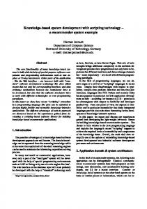
ST N is known to produce lots of spikes with high amplitude and also has loud background noise. It can be expected that signals recorded from it would present elevated Root Mean Square Value. This parameter is, among others, also used for Bayesian calculations in [5]. RM S approach is much less computationally demanding than spike detection and can be easier available. It still requires calculation of a sum of squares for all samples from a given recording. Because all samples contribute to the resulting value, this method takes into account both background noise and spikes. If the signal is contaminated by artifacts, the method may produce falsely high RM S values. RM S based method as shown on Fig. 1(a) in a clear way assesses that anterior8 electrode is better than medial9 . RM S method defines clear dorsal10 border of the ST N at -3000 with subsequent increase of the RM S up to depth -3000. Such findings and predicted thickness (6 mm) agree with clinical observations found in [3].
5
Analysis of the percentile value – PRC
Spikes amplitude is by far greater than the background noise. Because of that one can find an amplitude value below which no spikes are present or above which spike must rise. This feature is commonly used in many neurological appliances, for example the 50th percentile - median of amplitude’s module is used for both spike detection and artifact removal process. The approach in which 50th percentile (median) of amplitude’s module together with other features is used for detecting increased neural activity can be found in [9]. High amplitude ranges that comes from spikes lie after the 95th percentile. Certain percentile value calculated from module of amplitude can thus be used to estimate the amount of background neural activity. Already the 95th percentile shows background activity and discards almost all samples from the spikes. To be however safely independent from any spike activity, even lower percentile can be used. In this paper the 80th percentile is used. Having selected that percentile as a value that can be used for ST N distinguishing an electrode comparison chart can be made. Using the same data set that was used for creation of Fig. 1(a), we obtained following results (Fig. 1(b)). Obtained results are in full agreement with those 8 9 10
being most forward, closest to facial plane placed to the left/right side of the central electrode top
Foundations of system for localization of STN in PD patients.
5
given by RM S method. Both methods state that the best electrode is anterior and that ST N ranges roughly between -3000 and +3000. Decrease of percentile value is somewhat more steep than in the case of RM S, which a bit more clearly identifies the ventral11 border of the ST N .
6
DWT based analysis of the LF B power
It has been postulated in [12] and [11] that background neural activity can be divided into two frequency areas. First, an activity in range below 500 Hz is called Low Frequency Background(LF B). In mentioned paper authors use properties of HF B to pinpoint ST N location. Here, in this section a LF B based method for finding the ST N is shown. As with Quantile based estimator, here too, it is very important to remove as much of the artifacts as possible. This is due to the fact that most of the power carried by such artifacts resides in range below 375Hz that if fully included in the described analysis. Before the transformation can be made, any spikes are removed from the raw MER recorded signal. Later to ensure removal of even highly distorted spikes, signal is also hard thresholded with value of 80th percentile. After artifacts and spikes have all been removed, signal has to be firstly transformed from time to frequency domain. For this DWT is used. DWT is performed fully, i.e. all available forward steps are done. As the result, following list of wavelet coefficient sets is produced: cAn , cDn , cAn−1 , ... , cD1 . Each set of coefficients corresponds to specific frequency range. Signal’s power is subsequently calculated from all sets representing frequencies below 500 Hz. Once again the LF B power was calculated for the same set of electrodes that were used in previous sections. Results containing LF B power for electrodes and depths are shown on Fig. 1(c). Obtained results are in full agreement with those given by RM S and percentile methods. All methods state that best electrode is anterior. LF B based method localizes ST N between -3000 and +3000. This yields thickness of about 5mm which is in accordance with brain anatomy [2]. What is especially worth mentioning is the visible division of ST N into two different parts. Dorsal part spans -3000 to 0 and has lower power output. Ventral part spans from 0 to +1000 and is definitively more active. This finding agrees with [3].
7
DWT based analysis of the HF B power
In this section a modified version of the HF B calculation described in [12] and [11] is presented. Modification comes from the use of DWT based filtering. All principles regarding calculation of HF B and LF B are the same, only difference lies in frequency range. For HF B inspected frequency range is between 500 and 3000 Hz. After calculating HF B for test set of electrodes results shown on Fig. 1(d) were obtained. Ones again, obtained results are in full agreement with those given by RM S, percentile and LF B methods. There is however notable difference, HF B does not show subdivisions of ST N nucleus. 11
bottom
6
Konrad Ciecierski, Zbigniew W. Ra´s, Andrzej W. Przybyszewski
(a) RM S value chart (chap. 4) (b) 80th PRC chart (chap. 5)
(c) LF B chart (chap. 6)
(d) HF B chart (chap. 7)
Fig. 1. Results of RM S, P RC, LF B and HF B
8
Correlation between parallel electrodes recordings CORR
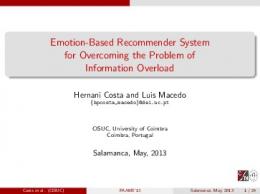
Authors in paper [6] and [7] suggest that increase in synchronization between neuronal networks in the basal ganglia contributes to clinical observations in PD i.e. rhythmic involuntary muscle movements. Paper [8] also states that phase between different adjacent layers of brain tissue may be inverted. Taking this into account MER data were converted to absolute values prior to DWT calculation. Having done such preprocessing, one can sometimes notice striking similarities between DWT of recordings coming from vicinity of the ST N . The synchrony appears to be most evident in frequencies below 23 Hz. Fig. 2 shows a DWT (part of cA9 ) transform of 2.7 s long recording from the ST N . Synchrony is not a natural phenomenon of the ST N and is only present in some cases of PD. It can not be so fully relied upon. Its presence on given depth implies high ST N probability. Its lack DOESN OT exclude ST N occurrence.
9
Comparison of methods
Summarizing previous sections, several different methods allowing localization of the ST N have been described. Each of the methods have some advantages and disadvantages. RM S and Percentile(P RC) based methods can be used for classification of single recordings. Their results can be however completely wrong if signal
Foundations of system for localization of STN in PD patients.
7
800 DWT value
600 400
Central Anterior Medial
200 0 −200 0
20
40
60
80
100
120
140
coefficient
Fig. 2. Synchronization in freq. below 23 Hz for ABS signal recorded in ST N
contains any artifacts. If the artifacts are present during the first five recordings, the Cbase (see section 2) can be set so high that the actual ST N location would not be detected at all. LF B and HF B based methods both rely on frequency analysis. They do not require prior filtering. In fact no prior filtering should take place. In some recording systems the frequencies below 500 Hz are automatically removed. When such recording is analyzed, the LF B method is of course unusable. In contrast to the previous methods, the CORR one does not work at single recording level. It looks for pair-wise similarities in recordings done by an array of electrodes at the same depth. With certain preprocessing (see section 8) this similarities indeed can be found in frequency range below 23 Hz. As mentioned in [6] and [7] such ST N synchrony is a hallmark of the PD. Unless caused by another illness it does not manifest in recording acquired from non-PD patients.
10
Recording clustering
Using the RM S, P RC, LF B and HF B methods, each recording d made by some electrode at given depth has the set of coefficients described by equation 1. C = {cRM S (d), cP RC (d), cLF B (d), cHF B (d)} (1) Having this coefficients, an attempt to obtain meaningful clustering of the recording has been done. Assumption was, that recordings can be divided into three clusters containing respectively: α – recordings made outside the ST N β – recordings made in areas near the ST N γ – recordings made inside the ST N Clustering has been done using hierarchical cluster tree with Euclidian distance and minimum variance algorithm. As input to the clustering procedure, all possible 2, 3 and 4 – element subsets of C has been tried. Regardless of the coefficients subset taken for clustering, the Spearman rank was greater than 0.86 and in many cases it is above 0.9. This ensures that produced clustering was of
8
Konrad Ciecierski, Zbigniew W. Ra´s, Andrzej W. Przybyszewski
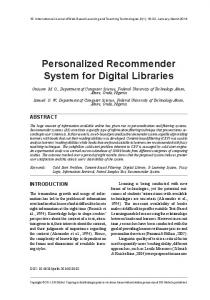
good quality. Cluster percentage size also seem to be stable. Having µα = 76.8, µβ = 17.4 and µγ = 5.8 and σα = 4.5, σβ = 4.1 and σγ = 2.4. 10.1 Cluster cross comparison On the following pictures some of the more interesting clustering results are shown. Especially interesting are the results obtained when clustering was made using one subset of coefficients and clustering results are also shown using another subset. Fig. 3(a) shows results of the clustering done using only coefficients cRM S and cHF B . One can clearly observe that data set has been divided into three sections. Cluster α – very dense and numerous, containing recordings assumed to be made outside of the ST N (6506 recordings). Cluster β – much less dense, containing recordings assumed to be made near the ST N (while having area similar to cluster A, it contains only around 1668 recordings). Cluster γ – sparse, containing recordings that are assumed to be coming from the ST N (contains only about 893 recordings). Fig. 3(b) shows results of the same clustering that is shown on Fig. 3(a). It shows however a recording seen from the point of view of other two coefficients (cP RC and cLF B ). One can plainly see the cluster α that contains recordings made outside ST N . As expected, the recording from that cluster have also small cP RC and cLF B values. Also, as expected, recordings from cluster γ are characterized by largest in population values of cP RC and cLF B . This is a clear evidence that obtained results are stable and regardless of chosen coefficient subset recordings are divided in a similar way. Taking C1 ⊆ C and C2 ⊆ C (see equation 1)
(a) Clustering with RM S and HF B shown on RM S, HF B plane
(b) Clustering with RM S and HF B shown on P RC, LF B plane
Fig. 3. Cluster cross comparison
the resulting α1 and α2 clusters in worst case scenario have over 96 % common elements. β1 and β2 clusters in worst case have over 75 % common elements. In case of γ clusters, the intersection in never below 78 %. Intersection between α
Foundations of system for localization of STN in PD patients.
9
and γ is never bigger than 0.07 %. This allows one to say with good certainty that obtained results are stable and comparable between clusterings. Recording that has been assigned with cluster label α is much, much less likely to come from the ST N than another one with cluster label β – even if labels come from different clusterings.
11
Review of clustering results
Let us introduce ranking between clusters. As our goal is to find the ST N , the most natural order is that α < β < γ. Having done that, assume that for a given recording, best cluster is the most favorable cluster among all assignments made by different clusterings. 11.1 Sample case Let us take the example pass of electrodes that was shown in section 4, 5, 6 and 7. Each electrode produced 16 recordings (from depths ranging -10000 µm to 5000 µm). Labels applied to all subsequent recordings of each electrode are shown in Clusters column of Table 1. Anterior electrode has five consecutive recordings labeled as γ and largest continuous β+ sequence (nine depths). Central electrode has three subsequent depth labeled as γ, they together with adjacent β recordings form 7 element sequence. M edial electrode has five depth labeled as γ, their largest sequence has 4 elements. γ together with adjacent β recordings form 7 element sequence. Basing on obtained results, as the best electrode we select the Anterior one – it contains largest sequence of γ labeled recordings. The 2nd best would be the M edial electrode, it contains as many γ recordings as the Anterior one albeit split into two subsequences. Having labeled the recordings, we can now offer a way to rank them as to how well did they reached / passed through the ST N . For this, we define three measures defined for an electrode: Mγ1 – count of recordings labeled as γ. Mγ2 – length of the longest sequence of recordings labeled as γ. Mγβ – length of the longest sequence of recordings labeled as γ or β. Electrodes are then ordered in descending order according to Mγ , Mγβ and finally to Mβ . Table 1. Electrode rank example Electrode Clusters Mγ1 Mγ2 Mγβ Anterior βααααααβγγγγγβββ 5 5 9 Medial αβαααααβγγγγβγαβ 5 4 7 Central αααααααααβγγγβββ 3 3 7
12
Summary of results
There are several ways in which given recordings can be classified as coming from ST N or not. They all have their advantages and disadvantages. Spike
10
Konrad Ciecierski, Zbigniew W. Ra´s, Andrzej W. Przybyszewski
based methods like meta power, intra spike histogram[3] or simple spike count must rely on spike detection. This can be difficult due to the nature of MER recorded signal. Low frequency components or artifacts can lead to incomplete detection of spikes. Also ST N is not the only area characterized by high spiking activity. This could led to both false negative and false positive detections of the ST N . Method basing on synchrony detection (see chapter 8) can provide some additional insight but are not very reliable. As explained they look for pathological ST N condition that does not have to occur. Last class of methods: RM S, P RC, LF B and HF B described in this paper do not directly rely on spike or synchrony detection. They do require some signal preprocessing. Especially essential is artifact removal. Each of them helps to find the ST N location using different approach, still, as pointed out in section 10 they greatly agree in their assessments. Hierarchical clusterings that base on the described methods proved to be an effective method for ST N discrimination. Obtained results are more stable, accurate and less probability dependant then those basing on spike detection. This all, proves that it is possible to construct autonomic and automatic decisive support system for ST N detection. Authors would like to thank Dariusz Koziorowski MD, PhD (Warsaw Medical University) and Tomasz Mandat, MD, PhD (Clinic of Neurosurgery at Warsaw Institute of Psychiatry and Neurology) for providing DBS recordings.
References 1. A.Jensen, A Ia Cour-Harbo. Ripples in Mathematics, Springer-Verlag 2001 2. J. Nolte. The Human Brain, Introduction to Functional Anatomy, Elsevier 2009 3. Z. Israel et al Microelectrode Recording in Movement Disorder Surgery, Thieme Medical Publishers 2004 4. Alexander B. et al Wavelet Filtering before Spike Detection Preserves Waveform Shape and Enhances Single-Unit Discr., J. Neurosci Methods. 2008, 34-40 5. A. Moran et al Real-Time Refinement of STN Targeting Using Bayesian DecisionMaking on the RMS Measure, J. Mvmt. Disorders. Vol. 21, No. 9, 2006, 1425-1431 6. R. Levy et al. Synchronized Neuronal Discharge in the Basal Ganglia of PD Patients Is Limited to Oscillatory Activity, J. Neuroscience, 2000, 7766-7775 7. A. Pogosyan et al. Parkinsonian impairment correlates with spatially extensive subthalamic oscillatory synchronization, J. Neuroscience 171, 2010, 245-257 8. Gyorgy Buzsaki et al High-Frequency Network Oscillation in the Hippocampus, Science 15 May 1992, Vol. 256 No. 5059, 1025-1027 9. P. Gemmar et al. MER Classification for DBS, 6th Heidelberg Innov. Forum, 2008 10. K. Ciecierski, Z. W. Ra´s, A. W. Przybyszewski Selection of the optimal electrode in Parkinson’s disease DBS treatment, Foundations of Intelligent Systems, ISMIS 2011 Symposium, LNAI, Vol. 6804, Springer, 2011, 554-564 11. P. Novak, A.W. Przybyszewski et al. Localization of the subthalamic nucleus in Parkinson disease using multiunit activity, J. Neur. Sciences 310, 2011, 44-49 12. P. Novak et al Detection of the subthalamic nucleus in microelectrographic recordings in Parkinson disease using the high-frequency (> 500 Hz) neuronal background, J. Neurosurgery 106, 2007, 175-179