FPGA-BASED IMPLEMENTATION OF A REAL-TIME 5000-WORD CONTINUOUS SPEECH RECOGNIZER Young-kyu Choi, Kisun You, and Wonyong Sung School of Electrical Engineering, Seoul National University San 56-1, Shillim-dong, Kwanak-gu, Seoul 151-744 Korea phone: +82-2-880-9372, fax: +82-2-882-4656, email: {ykchoi,ksyou}@dsp.snu.ac.kr,
[email protected] web: msl.snu.ac.kr
ABSTRACT We have developed a hidden Markov model based 5000word speaker independent continuous speech recognizer using a Field-Programmable Gate Array (FPGA). The feature extraction is conducted in software on a soft-core based CPU, while the emission probability computation and the Viterbi beam search are implemented using parallel and pipelined hardware blocks. In order to reduce the bandwidth requirement to external DRAM, we employed bit-width reduction of the Gaussian parameters, multi-block computation of the emission probability, and two-stage language model pruning. These optimizations reduce the memory bandwidth requirement for emission probability computation and inter-word transition by 81% and 44%, respectively. The speech recognition hardware was synthesized for the Virtex-4 FPGA, and it operates at 100MHz. The experimental result on Wall Street Journal 5k vocabulary task shows that the developed system runs 1.52 times faster than real-time. 1. INTRODUCTION Large vocabulary continuous speech recognition (LVCSR) is a complex task that requires much computation and data access. Hardware based speech recognition can deliver good performance while consuming relatively small power. There have been various hardware implementations of speech recognition algorithm. However, some are only partially hardware-designed and need additional external search units [1] [2], and some are adequate for only smallsized vocabulary [3] [4]. The recent work done by Lin et, al. [5] is a complete FPGA-based continuous speech recognizer. However, it can only support 1000-word vocabulary task and runs 2.3 times slower than real-time. The profiling result for hardware-based implementation of speech recognition reveals that the main bottleneck is the memory access, not computation. In the emission probability computation process, for example, the execution throughput of the computational part can be easily improved by using the pipelining technique. However, the required memory bandwidth for just this part is 286MB/s for real-time 5000-word continuous speech recognition. Most DDR SDRAM (Double Data Rate Synchronous DRAM) cannot support such memory bandwidth. Similarly, the computation for the search process is fairly straightforward since it conducts mostly compare and add operations. However this process spends much time for simply reading and updating the parameters stored in DRAM. An experiment on the 5000-word continuous speech recognition shows that 16,391 Hidden Markov Model (HMM) states and 71,711 word transitions must be
updated every frame, 10ms, on average. The observation explained above shows that the memory access time needs to be reduced to speed up the recognizer. In this paper, we propose a fine-grain pipelined hardware architecture which takes full advantage of the memory burst operation supported in DDR SDRAM. The execution time for computation overlaps with the memory latency in the developed architecture. We also present several memory access optimization techniques. We first reduced the bit-width of Gaussian parameters and devised a scheme to minimize the quantization error. Next, we proposed an efficient way of reusing the Gaussian parameters by computing the emission probability in multiple blocks. Finally, we utilized a two-level language model pruning technique to prohibit excessive memory reads and updates. The feature extraction part which requires a relatively small amount of computation is implemented using a softcore processor supported in the FPGA. This paper is organized as follows. Section 2 briefly describes the speech recognition algorithm used in this implementation. In Section 3, the architecture of the speech recognition hardware and its execution flow are explained. Several memory reduction techniques are explained in Section 4. Section 5 shows the experimental results, and the concluding remarks are made in Section 6. 2. SPEECH RECOGNITION SYSTEM OVERVIEW We have implemented a context-dependent HMM-based continuous speech recognizer [6]. The recognizer has three major parts - feature extraction, emission probability computation, and Viterbi beam search. The feature vector contains 39 elements, which consists of 13th order MFCC (Mel-Frequency Cepstral Coefficient), the delta, and the accelerator of the coefficients. The feature vector is computed for 30ms input speech frame at every 10ms. After the feature extraction, we can compute the probability of the feature vector being generated from the subphonetic HMM states. Each HMM state has an emission probability density function estimated during the acoustic model training. The emission probability for observation Ot of state s is approximated by the maximum Gaussian probability [7] as follows: log(b(Ot ; s)) = max{Cm − m
1 K (xk − µmk )2 ∑ σ 2 }, 2 k=1 mk
(1)
where K is the feature dimension and Cm is a Gaussian constant. µmk and σmk are means and variances of the Gaussian.
ψt (s j ; w) = max{ψt−1 (si ; w) + log(ai j )}
External DDR SDRAM Through 64-bit PLB Bus
BUS Master Data Storage
(2)
where ai j is the transition probability from the state i to j, and b(Ot ; s j , w) is the emission probability for the state j of the word w in the time frame t. ψt (s j ; w) is the accumulated likelihood of the most likely state sequence reaching the state j of the word w at time t. To reduce the search space, beam pruning is applied after the dynamic programming. Any state that has a smaller accumulated likelihood value than the beam threshold is discarded. Second, the inter-word transition based on the Eq. (3) is processed. The last state of each word propagates its accumulated likelihood to other words. The language model probability is incorporated in this procedure to give the constraint to the inter-word transition. We adopted the bigram language model, in which the probability of a word depends on the preceding word. The inter-word transition probability is computed as:
ψt (s0 ; w) = max{log(p(w|v)) + ψt (s f ; v)}, v
(3)
where p(w|v) is the bigram language model probability from word v to word w, s f indicates the final state, and s0 is the pseudo initial state. After detecting the end of the speech, the backtracking is performed to recover the recognition result. 3. FINE-GRAIN PIPELINED ARCHITECTURE 3.1 Overall Architecture The overall architecture of the implemented speech recognition system is shown in Fig. 1. The feature extraction is conducted at the master processor in software. Microblaze supported in the Virtex 4 FPGA is utilized as the master processor. It is possible to employ a different type of feature or enhance the recognition accuracy by preprocessing the input sound. Noise reduction or speaker adaptation can also be added in software. As shown in Fig. 1, the system consists of three parts - emission probability computation, dynamic programming & beam pruning, and language model pruning & inter-word transition units. The architecture of each unit will be described in detail throughout this section. In order to reduce external DRAM access, we used multiple internal Block RAMs (BRAMs). Table 1 shows the usage of BRAMs. Only frequently accessed data is stored in the BRAM, by which the bandwidth reduction is maximized. The size of one BRAM in Virtex-4 FPGA is 18Kbit. Due to the limitation on the size of available internal BRAMs, the large-sized data is stored in the external DRAM instead. The DRAM stores 4.91MB of Gaussian parameters, 699KB of HMM state parameters, and 3.23MB of language model probability and inter-word transition list.
Inter-word Transition
Updated Word Data
Word Data
HMM States Parameters
Write Buffer
i
+log(b(Ot ; s j , w)),
Language Model Pruning
Arc Data
Updated HMM States Parameters
Dynamic Programming
State Beam Pruning
Emission Prob.
Internal BRAM (308KB)
After computing the emission probability of all the HMM states, the best state sequence up to the current frame should be found in the search network. The time synchronous Viterbi beam search [8] is employed, which can be divided into two parts. First, we perform the dynamic programming (DP) recursion shown in Eq. (2) to obtain the best accumulated likelihood of the state sequence candidates.
Active Acoustic Model List Acoustic Model Data
Burst Controller
Emission Emission Probability Probability Computation Computation
Emission Prob.
Feature Data
Microblaze Microblaze
Figure 1: Overall Speech Recognition Architecture Table 1: Internal BRAM Utilization Emission Prob. Active Word List Inter Word Trans. HMM State Status Others Total
# of BRAM 32 10 48 28 19 137
Bandwidth (MB/s) 3.52 2.46 12.51 2.06 1.57 22.12
Unlike BRAM, it takes several cycles to access the external DRAM. To reduce the effect of such latency, we tried to exploit the burst operation of DRAM. The burst mode allows us to increase the throughput of memory access since the data can be accessed every cycle. To efficiently utilize the burst mode, we propose fine-grain pipelined architecture that can handle continuous stream of data. The proposed architecture can process one HMM state or one inter-word transition every clock cycle. By using this pipelined architecture, the computation time overlaps with the data access time. Such scheme allowed us to effectively use the DRAM despite the long latency. 3.2 Emission Probability Computation Unit The emission probability computation unit calculates the likelihood log(b(Ot ; s)) of the HMM state s. The Gaussian parameters, the mean µmk and the standard deviation σmk are sequentially read from the DRAM. Then this unit compares µmk and σmk with the feature data Ot , and computes its emission probability. The computation is performed in 4 stages: subtraction, multiplication, multiplication, and accumulation. The pipelined architecture for emission probability computation is commonly used in many hardware-based speech recognizers [1] [2] [5] [9]. After the computation has been finished, the emission probability is stored in the internal BRAM. Then, this value is used by the dynamic programming unit to determine the likelihood of each HMM state. 3.3 Dynamic Programming & Beam Pruning Unit Dynamic programming recursion shown in Eq. (2) is performed to evaluate the accumulated likelihood of HMM states. The pipelined architecture proposed in [9] is not feasible for 5000-word recognition since it requires a much larger internal BRAM. Our proposed architecture, on the
Pass
Threshold >
Likelihood (state 2)
+ +
Emission Probability
Pass
Buffer
> + +
Stage 1
Stage 2
CLK
State 2 Info
State Info Write (to DRAM Write Buffer )
State 3 Info
State 4 Info
State 5 Info
State 6 Info
1 : Accum. Likelihood Update
2 : NOP
3 : NOP
4 : Accum. Likelihood Init
State 7 Info
Emission Prob. Read Request (to BRAM)
1 : Emission Prob. Read Req
2 : NOP
3 : NOP
4 : Emission Prob. Read Req
5 : Emission Prob. Read Req
6 : Emission Prob. Read Req
Stage 1 Computation
1 : Accum. Likelihood CMP
2 : NOP
3 : NOP
4 : Accum. Likelihood CMP
5 : Accum. Likelihood CMP
6 : Accum. Likelihood CMP
1 : Emission Prob. ADD & Thres. CMP
2 : NOP
3 : NOP
4 : Emission Prob. ADD & Thres. CMP
5 :Emission Prob. ADD & Thres. CMP
1 : NOP
2 : Validate
3 : NOP
4 : Invalidate
Stage 2 Computation
HMM State Status Update
color index (prev HMM state status ) -> (next HMM state status )
:
Act -> Act
Read Req >
Inact -> Act
Inact -> Inact
Enable
Buffer
+
LM Threshold Stage 2
Figure 4: Pipelined Execution of Language Model Pruning & Word Update Unit
Stage 3
Figure 2: Pipelined Execution of Dynamic Programming & Beam Pruning Unit
State 1 Info
Language Model Probability (arc 1)
Word Address
Stage 1
Likelihood Buffer
State Info Read (from DRAM)
Next Word Address (arc 1)
Last State Likelihood
MUX
DRAM
BRAM Reader
Updated State Likelihood +
Likelihood (state 1)
> +
Init
>
Likelihood Buffer
Language Model Probability (arc 2)
>
MUX
Buffer
Word Address
BRAM Writer Updated First State Likelihood
Emission Probability
+ Buffer
MUX
DRAM
>
Next Word Address (arc 2)
Transition Likelihood
+ Likelihood Buffer
BRAM Reader
Threshold
Read Req
+
DRAM Write Buffer
From DRAM
Likelihood (state 3)
State status
Buffer
First State Likelihood of the Next Word
>
MUX
DRAM
Pass
Buffer
From DRAM
Likelihood Buffer
Act -> Inact
Figure 3: Timing Diagram of the Pipelined Execution
other hand, is DRAM-based, and efficiently uses the burst mode of DRAM. The architecture is shown in Fig. 2, and its pipeline timing diagram is described in Fig. 3. In the first stage, the likelihood from the current state is compared with that from the previous state. If the HMM state was active, the higher likelihood between the two is selected and stored in a buffer for the next cycle. Also, the request signal for the emission probability that corresponds to the current HMM state is sent to the BRAM in this stage. If the HMM state was inactive, an ’NOP’ is inserted in the pipeline since it is unnecessary to perform the comparison between the likelihood of the current state and that of the previous state. This can be seen in the State 3 of Fig. 3. In the second stage, the emission probability requested from the first stage is available. Therefore, the stored likelihood in the previous stage can be added to the emission probability. Then, this added value is compared with the beam threshold value. If it is bigger than the threshold, the updated
likelihood value is sent to the third stage as in State 1 of Fig. 3. If the result is smaller than the threshold, the ’init’ signal shown in the the second row of Stage 2 in Fig. 2 is sent to the third stage. In the third stage, the updated likelihood from the second stage is written to the DRAM write buffer. If the ’init’ signal was sent from the second stage, an initialized value is instead written to the write buffer. The updated likelihood values in the write buffer are written to the DRAM in a burst mode when the write buffer becomes full. Also, the state status is updated in this stage. If the accumulated likelihood in the second stage is bigger than the beam threshold, it stays active, as in the State 1 of Fig. 3. If not, it becomes inactive, as in the State 4 of Fig. 3. An exceptional case would be when the previous state is active, but the current state is inactive. In this case, the current state becomes active in the next time frame. This is shown in the State 2 of Fig. 3. Since each stage is independent of others, the next HMM state can be processed after one cycle in the same manner explained above. Such fine-grain pipeline architecture allows us to overlap the computation time with the memory access delay, and makes it possible to efficiently utilize the burst operation capability of DRAM. 3.4 Language Model Pruning & Inter-word Transition Unit After updating all HMM state parameters, the inter-word transition probability is computed. Our implementation method is slightly different from Eq. (3), in that Eq. (3) selects the maximum probability by traversing through the incoming transition, but we chose to update the probability by checking the outgoing transition. The final result would be the same, but the difference is that direct implementation of Eq. (3) would sometimes result in accessing an inactive last state. Our implementation style is more regular since the first state of the receiving word is always active. The architecture of this unit is shown in Fig. 4. The language model probability and the next word address are read from the DRAM. In the first stage, the language model probability is added to the likelihood of the last state. Then the result is compared with the language model threshold. If it is bigger than the language model threshold,
Table 2: Memory Bandwidth Reduction with Bit-width Optimization Bit-width 16-bit 8-bit Optimized 8-bit
WER (%) 9.19 31.55 9.36
Bandwidth (MB/s) 286.4 386.1 145.7
a read request signal for the likelihood value of the first state of the next word is asserted. Also, the transition probability is stored in a buffer for the second stage. In the second stage, the likelihood value of the first state of the next word is available. This value is compared with the inter-word transition probability from the first stage. If the inter-word transition probability is larger than the likelihood of the first state, the likelihood of the first state is updated with the new transition probability. If it is smaller, it is not updated. The operations in the Stage 1 and the Stage 2 are independent with each other. Therefore, these processes can be executed in a pipelined manner. Similar to the dynamic programming unit, this pipelined architecture allows us to efficiently use the burst mode of DRAM and hide the computation in the memory access time. 4. MEMORY BANDWIDTH REDUCTION As mentioned in Section 1, a real-time large vocabulary speech recognition system requires a large number of memory accesses. Therefore, we tried to reduce the memory bandwidth requirement of the system as explained in this section. 4.1 Bit-width Reduction of Gaussian Parameters The emission probability computation part of the baseline system requires a high memory bandwidth of 286.4MB/s for real-time processing. Since it adopted 16-bit Gaussian parameters, we first simply reduced the bit-width of means and variances to 8 bits. However, it became harder to differentiate the likelihood of the HMM states as the quantization error increased. As a result, the recognizer had to search and compare wider number of state sequences. The memory requirement increased as shown in Table 2. The quantization error is reduced by two methods. First, the standard deviation was used instead of the variance. The standard deviation needs a smaller dynamic range than the variance. Second, the means and the standard deviations with similar dynamic range were grouped together. The 13 MFCC coefficients, their delta, and the accelerator employ different quantization schemes. After applying these two techniques, we were able to reduce the memory bandwidth by 49.1% while losing the Word Error Rate (WER) by 0.17% as shown in Table 2. 4.2 Multi-block Computation for Gaussian Parameter Reuse We computed the emission probability of four frames in parallel. Although this technique introduces a small delay of 40 ms, it makes it possible to reuse the Gaussian parameters and reduce the DRAM access. A similar reuse technique proposed in [2] computes the probability of all HMM states. However, this is inefficient because only 30.4% of HMM
states are active, on average. Our recognizer, on the other hand, computes the probability of only active HMM states. At the end of every four frames, the emission probability of active HMM states for four frames is computed in parallel, and the result is stored in the BRAM along with a list of active HMM states. An HMM state that becomes active in the middle of four frames has to look up the active HMM state list. If it is not in the active list, the emission probability of that HMM state is computed in the middle of four frames. Since the active HMM state list changes from frame to frame, it is not possible to achieve an ideal bandwidth reduction of 75%. Nonetheless, the recognizer still reduces 66.8% of DRAM access, since an active HMM state tends to stay active in adjacent frames. The memory bandwidth became 48.3MB/s without losing the accuracy. 54KB of additional BRAM was used to store the emission probability. Note that it is also possible to further decrease the memory bandwidth by extending the number of parallel-computed frames at the cost of additional BRAM. 4.3 Two-stage Language Model Pruning If the pruning threshold can be estimated before starting the computation, the pruning can be performed immediately after obtaining the new language model probability. Then we can avoid updating the inter-word transitions that have the probability below the threshold. A beam pruning method with similar approach was proposed in [5]. For further improvement, we propose two-stage language model pruning. For each word v, the highest language model probability maxw {log(p(w|v))} among the transitions is stored in the BRAM in advance. In the first stage, the best transition language model probability {maxw {log(p(w|v)} + ψt (s f ; v)} is compared with the language model pruning threshold. If the best transition probability does not exceed the threshold value, it is certain that the rest of transition probability would not exceed it, either. Therefore, the rest of the language model probability and its corresponding next node address is not fetched from the DRAM. However, if the best transition probability is bigger than the threshold value, it means that some transition probability would be bigger than the threshold. Thus, the transition information is read from the DRAM. The transition probability is then computed and compared with the pruning threshold in the second stage. Our proposed method further reduces the DRAM bandwidth of inter-word transition part from 23.7MB/s to 12.8MB/s. 5. EXPERIMENTAL RESULTS 5.1 Experimental Setup We used Xilinx’s Evaluation Board ML402 [10] as the target platform. It has a Virtex-4 SX35 FPGA which provides 432KB of internal BRAM, 32-bit wide 64MB DDR SDRAM, and various peripherals. The speech recognition hardware and the DDR SDRAM are connected to the PLB bus, which has a width of 64 bits and supports a burst length of 16. The speech recognition hardware and the external DDR SDRAM operates at 100MHz. The acoustic model of the recognition system was trained by HTK, an open-source speech recognition toolkit [11]. The speaker independent training data in Wall Street Journal 1 corpus is used. The acoustic model data consists of 7,862 shared HMM states. Each state has a mixture of eight
200 Inter-word Transition 180 Dynamic Programming 160 Emission Prob.
MCycles/s
140 120
Real-time
100
tecture to efficiently utilize the burst operation of the external DRAM. We also applied several memory access reduction techniques such as the bit-width reduction of Gaussian parameters, the multi-block computation of emission probability, and the two-stage language model pruning. The memory access reduction techniques lead to 2.77 times speed-up in execution cycles.
80
7. ACKNOWLEDGEMENT
60 40
This work was supported in part by the Brain Korea 21 Project and ETRI SoC Industry Promotion Center, Human Resource Development Project for IT SoC Architect.
20 0 Baseline
Bit-width Opt.
Gaussian Parameter Reuse
Two-stage LM Pruning
REFERENCES Figure 5: Execution Clock Cycle Requirement of the Recognizer Table 3: FPGA Synthesis Result Unit Slices Slices FFs LUTs RAMB16s DSP48s
Recognizer HW 4,470 (29%) 4,543 (15%) 7,794 (25%) 137 (71%) 17 (9%)
Microblaze & Etc 5,106 (33%) 3,372 (11%) 6,424 (21%) 38 (20%) 3 (2%)
Total 9,576 (62%) 7,915 (26%) 14,218 (46%) 175 (91%) 20 (10%)
Gaussian distributions. For the evaluation of the system, we performed Wall Street Journal 5k-word continuous speech recognition task. The test set consists of 330 sentences spoken by several speakers. The language weight is set to 16.0 and the word error rate of the implemented system is 9.36%. 5.2 Execution Time We analyzed the execution time of the recognition system with respect to various memory reduction schemes shown in Section 4. The clock cycles taken by the speech recognizer to process 330 sentences were divided by the time length of all the speech samples. Fig. 5 shows the change in execution cycles after applying the optimization techniques. The final system is about 2.77 times faster than the baseline. Note that the execution cycles of the dynamic programming do not vary in this experiment because the baseline system is already optimized with the proposed pipelined architecture. The real-time factor of the final system is 0.66. 5.3 Synthesis Result The FPGA synthesis result of the speech recognition system is shown in Table 3. Since we adopted internal BRAM to store internal data variables, the utilization factor of the BRAM block (RAMB16s) is rather high (91%). However, there are many hardware slices left which gives us the chance to add several features such as hardware based feature extraction and adaptive microphone beamforming in the future. 6. CONCLUDING REMARKS We have implemented an FPGA-based 5000-word continuous speaker-independent speech recognizer that satisfies the real-time constraint. We proposed fine-grain pipelined archi-
[1] U. Pazhayaveetil, D. Chandra, and P. Franzon, “Flexible low power probability density estimation unit for speech recognition,” IEEE Int. Symp. on Circuits and Systems (ISCAS), pp. 1117–1120, 2007. [2] B. Mathew, A. Davis, and Z. Fang, “A low-power accelerator for the SPHINX 3 speech recognition system,” Int. Conf. on Compilers, Architecture and Synthesis for Embedded Systems (CASES), pp. 210–219, 2003. [3] S. Nedevschi, R. Patra, and E. Brewer, “Hardware speech recognition for user interfaces in low cost, low power devices,” 42nd Annual Conf. on Design Automation (DAC), pp. 684–689, 2005. [4] R. Kavaler, M. Lowy, H. Murveit, and R. Brodersen, “A dynamic-time-warp integrated circuit for a 1000-word speech recognition system,” IEEE Journal of SolidState Circuits, vol. 22, no. 1, pp. 3–14, Feb. 1987. [5] E. Lin, Y. Kai, R. Rutenbar, and T. Chen, “A 1000-word vocabulary, speaker independent, continuous live-mode speech recognizer implemented in a single FPGA,” ACM/SIGDA 15th Int. Symp. on FPGA, pp. 60–68, 2007. [6] X. Huang, A. Acero, and H. W. Hon, Spoken Language Processing - A Guide to Theory, Algorithm, and System Development. Prentice Hall PTR, New Jersey, 2001. [7] B. Pellom, R. Sarikaya, and J. Hansen, “Fast likelihood computation techniques in nearest-neighbor based search for continuous speech recognition,” IEEE Signal Processing Letters, vol. 8, no. 8, pp. 221–224, August 2001. [8] H. Ney and S. Ortmanns, “Dynamic programming search for continuous speech recognition,” IEEE Signal Processing Magazine, pp. 64–83, 1999. [9] J. Schuster, K. Gupta, R. Hoare, and A. K. Jones, “Speech silicon: An FPGA architecture for realtime hidden markov-model-based speech recognition,” EURASIP Journal on Embedded Systems, vol. 2006, pp. 1–19, 2006. [10] Xilinx, ML401/ML402/ML403 Evaluation Platform UG080. http://www.xilinx.com, 2006. [11] S. Young, G. Evermann, D. Kershaw, G. Moore, J. Odell, D. Ollason, V. Valtchev, and P. Woodland, The HTK Book Version 3.3, 2005.