Frequent Pattern Mining with Uncertain Data ∗
Charu C. Aggarwal
IBM T. J. Watson Research Ctr Hawthorne, NY, USA
[email protected] †
Jianyong Wang
Tsinghua University Beijing, China
[email protected]
Yan Li Tsinghua University Beijing, China
[email protected] Jing Wang New York University New York, NY, USA
[email protected]
ABSTRACT
1. INTRODUCTION
This paper studies the problem of frequent pattern mining with uncertain data. We will show how broad classes of algorithms can be extended to the uncertain data setting. In particular, we will study candidate generate-and-test algorithms, hyper-structure algorithms and pattern growth based algorithms. One of our insightful observations is that the experimental behavior of different classes of algorithms is very different in the uncertain case as compared to the deterministic case. In particular, the hyper-structure and the candidate generate-and-test algorithms perform much better than tree-based algorithms. This counter-intuitive behavior is an important observation from the perspective of algorithm design of the uncertain variation of the problem. We will test the approach on a number of real and synthetic data sets, and show the effectiveness of two of our approaches over competitive techniques. Executable and Data Sets: Available at: http://dbgroup.cs.tsinghua.edu.cn/liyan/u mining.tar.gz
Data mining of uncertain data has become an active area of research recently. A detailed survey of uncertain data mining techniques may be found in [2]. In this paper, we will study the problem of frequent pattern mining with uncertain data. The problem of frequent pattern mining with uncertain data has been studied in a limited way in [7, 8, 11, 14], and a variety of pruning strategies are proposed in order to speed up the algorithm for the uncertain case. This paper will study the problem of frequent pattern mining by examining the relative behavior of the extensions of well known classes of deterministic algorithms. Since many of the techniques used across different frequent pattern mining algorithms are similar, the methodologies for extending the different algorithmic classes have will have applicability beyond the specific algorithms discussed in this paper. One observation from our extensions to the uncertain case is that the respective algorithms do not show similar trends to the deterministic case. For example, in the deterministic case, the FP-growth algorithm is well known to be an extremely efficient approach. However, in our tests, we found that the extensions of the candidate generate-and-test as well as the hyper-structure based algorithms are much more effective. Furthermore, many pruning methods, which work well for the case of low uncertainty probabilities do not work very well for the case of high uncertainty probabilities. This is because the extensions of some of the algorithms to the uncertain case are significantly more complex, and require different kinds of trade-offs in the underlying computations. Thus, in addition to the new efficient methods proposed by this paper, an important contribution of this paper is the insight that natural extensions of deterministic algorithms may show counter-intuitive behavior. This paper is organized as follows. The next section defines the uncertain version of the problem. We will also discuss the extension of candidate generate-and-test algorithms to the uncertain version of the problem. The remainder of the paper discusses the extension of other classes of algorithms, and provides comparative experimental results.
Categories and Subject Descriptors H.2.8 [Information Systems]: Database Applications
General Terms Algorithms ∗This research is continuing through participation in the International Technology Alliance sponsored by the U.S. Army Research Laboratory and the U.K. Ministry of Defense. †Jianyong Wang was supported in part by Basic Research Foundation of Tsinghua National Laboratory for Information Science and Technology (abbr. TNList), and the Program of State Education Ministry of China for New Century Excellent Talents in University under Grant No. NCET-070491, and a research award from Google, Inc.
Permission to make digital or hard copies of all or part of this work for personal or classroom use is granted without fee provided that copies are not made or distributed for profit or commercial advantage and that copies bear this notice and the full citation on the first page. To copy otherwise, to republish, to post on servers or to redistribute to lists, requires prior specific permission and/or a fee. KDD’09, June 28–July 1, 2009, Paris, France. Copyright 2009 ACM 978-1-60558-495-9/09/06 ...$5.00.
1.1 Contributions of this Paper This paper extends and compares many of the conventional techniques for frequent pattern mining to the uncertain case. These include candidate generate-and-test algorithms, hyper-structure based algorithms, and pattern-
growth algorithms. While the problem of uncertain frequentpattern mining has recently been studied in a limited way in the literature [8, 14], this is the first comprehensive study which proposes extensions of many classes of algorithms to the uncertain case. In addition to the efficient algorithms proposed, our results suggest that the behavior of the natural uncertain extensions of frequent pattern algorithms is quite different from the deterministic case. The results of this paper suggest for the first time that the efficiency and memory trade-offs are very different for the uncertain case, and it is important to pick the algorithms carefully for extension to uncertain data sets. Since the observations of this paper are fairly general, they may also help in designing better extensions of other deterministic algorithms to the uncertain case.
the product of the corresponding probabilities. Therefore, we have the following relationship: Y p(i, T ) (1) p(I, T ) =
2.
2.1 Candidate Generate-and-Test Algorithms
FREQUENT PATTERN MINING OF UNCERTAIN DATA SETS
In this section, we will discuss frequent pattern mining for uncertain data sets. We first introduce some additional notations and definitions. We assume that we have a database D containing N transactions. We assume that the total number of unique items is d, and each item is denoted by a unique index in the range of {1 . . . d}. In sparse databases, only a small number of items have a nonzero probability of appearing in a given transaction. Let us assume that the ith transaction in database D contains ni items with non-zero probability. Let us assume that the items in the ith transaction are denoted by j1i . . . jni i . Without loss of generality, we can assume that these items are in sorted order. We assume that the probability of the ith item being present in transaction T is given by p(i, T ). Thus, in the uncertain version of the problem, the item may be present in the transaction T with the above-mentioned probability. First, we will define the frequent pattern mining problem. Since the transactions are probabilistic in nature, it is impossible to count the frequency of itemsets deterministically. Therefore, we count the frequent itemsets only in expected value. In order to do so, we need to count the probability of presence of an itemset in a given transaction. Let s(I) be the support of the itemset I. This support can only be counted in probabilistic value. The expected support of an itemset I is defined as follows: Definition 2.1. The expected support of itemset I is denoted by E[s(I)], and is defined as the sum of the expected probabilities of presence of I in each of the transactions in the database. The problem of frequent itemset mining is defined in the context of uncertain databases as follows: Definition 2.2. An itemset I is said to be frequent when the expected support of the itemset is larger than the userdefined threshold minsup. Note that the expected number of occurrences of the itemset I can be counted by summing the probability of presence of the itemsets in the different transactions in the database. The probability of the presence of itemset I in a given transaction can be computed using the relationship below. Observation 2.1. The probability of the itemset I occurring in a given transaction T is denoted by p(I, T ) and is
i∈I
The above observation assumes statistical independence between the different items in terms of their uncertain probability behavior, which is the same as the assumption in other related work [7, 8]. This is also a widely used simplifying assumption across other data mining applications [2]. This does not mean that the underlying instantiations of such a database will result in uncorrelated items, since the values of p(i, T ) may be non-zero in a transaction only across a small fraction of correlated items.
We first study candidate generate-and-test algorithms for frequent pattern mining. These can be join-based [3] or setenumerations based [1]. The conventional Apriori algorithm [3] belongs to this category. The Apriori algorithm uses a candidate generate-and-test approach which uses repeated joins on frequent itemsets in order to construct candidates with one more item. A key property for the correctness of Apriori-like algorithms is the downward closure property. We will see that the downward-closure property is true in the uncertain version of the problem as well. Lemma 2.1. If a pattern I is frequent in expected support, then all subsets of the pattern are also frequent in expected support. Proof. Let J be a subset of I. We will first show that for any transaction T , p(J, T ) ≥ p(I, T ). Since J is a subset Q p(I,T ) of I, we have p(J,T = i∈I−J p(i, T ) ≤ 1. This implies that ) p(J, T ) P ≥ p(I, T ). Summing P this over the entire database D, we get T ∈D p(J, T ) ≥ T ∈D p(I, T ). Therefore, we have: E[s(J)] ≥ E[s(I)] The result follows. The maintenance of the downward closure property means that we can continue to use the candidate-generate-and-test algorithms without the risk of losing true frequent patterns during the counting process. In addition, pruning tricks (such as those discussed in Apriori) which use the downward closure property can be used directly. Therefore the major steps in generalizing candidate generate-and-test algorithms are as follows: (1) All steps for candidate generation using joins and in pruning with the downward closure property remain the same. (2) The counting procedure needs to be modified using Observation 2.1. We note that a number of recent techniques [7, 8] use further pruning tricks in order to improve efficiency. We will show that the effectiveness of such techniques is datadependent, since such pruning tricks do not work very well in the case of dense data sets in which uncertainty probabilities are high. Similar techniques can be used in order to extend setenumeration based methods [1, 4, 6]. These methods typically use top-down tree-extension in conjunction with branch validation and pruning using the downward closure property. Different algorithms use different strategies for generation
of the tree in order to obtain the optimum results. Since the set-enumeration based algorithms are also based on the downward closure property, they can be easily extended to the uncertain version of the problem. The key modifications to set-enumeration based candidate generate-and-test algorithms are as follows: (1) The tree-extension phase uses the ordering of the different items in order to construct it in top-down fashion. The tree extension phase is exactly the same as in candidate generate-and-test algorithms. (2) The counting of frequent patterns uses Observation 2.1. (3) In the event that transactions are projected on specific branches of the tree (as in [1]), we can perform the projection process, except that we need to retain the probabilities of presence of specific items along with the transactions. Also note that the probabilities for the items across different transactions need to be maintained respectively, even if the transactions are identical after projection. This is because the probabilities of the individual items will not be identical after projection. Therefore each projected transaction needs to be maintained separately. (4) The pruning of the branches of the tree remains identical because of the downward closure property.
3.
PATTERN GROWTH ALGORITHMS
There are also some popular frequent pattern mining algorithms, which are based on the pattern growth paradigm. Among these methods, the H-mine [12] and FP-growth [9] algorithms are two representative ones. Their main difference lies in the data representation structures. FP-growth adopts a prefix tree structure while H-mine uses a hyperlinked array based structure. We will see that the use of such different structures have a substantially different impact in the uncertain case as compared to the deterministic case. Next, we will discuss the extension of each of these algorithms to the uncertain case in some detail. a
H eader table H
H yper-linked array
c
d
e
g
2.3 2.1 2.8 2.4 1.4
c
0.7
d
0.8
e
0.7
g
0.6
a
0.8
c
0.7
d
0.6
e
0.9
a
0.7
d
0.6
e
0.8
g
0.8
a
0.8
c
0.7
d
0.8
Figure 1: H-Struct
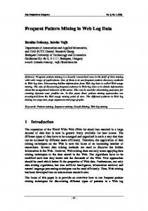
3.1 Extending the H-mine algorithm The H-mine algorithm proposed in [12] adopts a hyperlinked data structure called H-struct. Similar to FP-growth, it is a partition-based divide-and-conquer method. Initially, H-mine scans the input database once to find the frequent items. The infrequent items are removed from the database. The frequent items left in each input transaction are sorted according to a certain global ordering scheme. The transformed database is stored in an array structure, where each row corresponds to one transaction. During the mining process, there always exists a prefix itemset (denoted by P , which is initially empty). H-mine needs to construct a
header table which records the starting places of the projected transactions. By following the links in the header table, H-mine can locate all the projected transactions and find the locally frequent items by scanning the projected transactions. The locally frequent items w.r.t the prefix P can be used to extend P to longer prefix itemsets. As the hyper-linked array structure used in H-mine is not in a compressed form, it is relatively easy to extend the H-struct for mining frequent itemsets from uncertain data. As described in [12], each frequent item in a transaction is stored in an entry of the H-struct structure with two fields: an item id and a hyper-link. In addition, the probability p(i, T ) of the presence of item i in transaction T is maintained. Figure 1 shows an example of an extended H-struct structure1 . With the extended H-struct structure there are two ways to mine frequent itemsets with the current prefix P . The first approach is to maintain the probability p(P, T ) of prefix P occurring in each projected transaction T in memory. As the probability of the presence of locally frequent item i in transaction T is recorded in the extended H-struct, it is straightforward to compute the expected support of the new itemset of P ∪{i}, E[s(P ∪{i})], according to Observation 2.1 and Definition 2.1. However, the expected support of prefix P with respect to each conditional transaction needs to be maintained until all the locally frequent items w.r.t. prefix P have been processed. This may cost significant memory and may also lead to deterioration in the internal caching behavior of the algorithm. In order to avoid maintaining the probability of prefix P with respect to each projected transaction T , p(P, T ), we have another approach for computing it on the fly. As Hmine adopts the pseudo-projection method, each original input transaction is stored in the H-struct. By scanning the sub-transaction before the projected transaction of prefix P , we can find the probability of each item in P . Thus, p(P, T ) can be computed according to Observation 2.1. In a similar way, E[s(P ∪ {i})] can be computed according to Observation 2.1 and Definition 2.1. In this paper, we adopt the second approach for computing the expected support of the current prefix itemset P . This is because the use of onthe-fly computations reduces the space-requirements of the technique. The reduced space-requirements also indirectly improve the locality of the caching behavior of the underlying computations. This leads to improved efficiency of the overall algorithm.
3.2 Extending the FP-growth Algorithm FP-growth [9] is a key frequent itemset mining algorithm, which is based on the pattern growth paradigm. It adopts a prefix tree structure, FP-tree, to represent the database (or conditional databases). As FP-tree is a compressed structure, it poses several challenges when we try to adapt the FP-growth algorithm for uncertain data sets. These challenges are as follows: (1) In the original FP-tree structure, each node has a ‘count’ entry which records the number of transactions containing the prefix path from the root node to this node. For uncertain data, if we just store in a node the sum of item probabilities with respect to the transactions containing the prefix path, we will no longer be able to determine the prob1
Note that the second row of the header table in the Hstruct structure stores the sum of item probabilities for each locally frequent item.
ability of the presence of an item in each transaction. Thus, there is an irreversible loss of information in the uncertain case with the use of a compressed structure. Thus, we need to find a different and efficient way to store the item probabilities without losing too much information. (2) The original FP-growth algorithm mines frequent itemsets by searching the tree structure in a bottom up manner. The computation of the support of a given prefix path is quite straightforward. Its support is simply the support of the lowest node of the path. However, for uncertain data, the expected support of a given prefix path should be computed according to Definition 2.1. As we no longer know the mapping among the item probabilities and the transactions, it is impossible to compute the exact expected support of a given prefix according to Definition 2.1. (3) Since it is impossible to determine the exact expected support of each frequent itemset based on the FP-tree structure, we may need to first mine all the candidate itemsets, and then remove the infrequent itemsets by checking the original database. The process of determining such infrequent itemsets efficiently can be quite difficult in the uncertain case. There are two extreme solutions to adapt the FP-tree structure for uncertain data mining. Let us denote the FPtee built from uncertain data by UFP-tree. The first one is to store (in each node) the sum of item probabilities with respect to the transactions containing the prefix path from the root to it. The UFP-tree built in this way is as compact as the original FP-tree. However, it cannot even be used to compute the the upper bound or lower bound of the expected support of an itemset, because it loses information with respect to the distinct probability values for different transactions. Another extreme solution is to split a node into m nodes if the item in this node has m distinct probability values. In this case, we can compute the exact expected support. On the other hand, the UFP-tree built in this way consumes a lot of memory. In this work, we adopt a compromise by storing a subset of the probabilities for the item in each node. These probabilities are selected using clustering, and are stored as floating point numbers. This method does not consume too much memory, and we will show that it allows us to compute an upper bound on the expected support of any itemset. We then compute a set of candidate frequent itemsets based on this upper bound. This set of candidates provides us with a superset of the complete set of real frequent itemsets. Any remaining false positives will then need to be removed by scanning the input database. Next, we will discuss the adaptation of different steps of the FP-growth algorithm to the uncertain case.
3.2.1 Construction of the UFP-tree The process of constructing the UFP-tree for uncertain data is very similar to the construction of the FP-tree for deterministic data sets. The main difference lies in the information stored in each node. The UFP-tree is built using the following steps. First, the database is scanned to find the frequent items and to generate a support descending item list. Then, the transactions are read one by one, and the infrequent items are pruned. The remaining frequent items are sorted according to the frequent item list. The re-ordered transactions are inserted into the UFP-tree. As discussed earlier in this paper, each node of the UFP-
tree stores a summary of the probabilities of the non-zero probability items in those transactions which share the same prefix path in clusters. We partition the probabilities into a set of k clusters. The corresponding parameters created for the ith cluster by the partitioning are represented by ci and mi (1 ≤ i ≤ k), where ci denotes the maximum probability value in the ith cluster and mi is the number of item probabilities in the ith cluster. We assume that c1 > c2 > . . . > ck . The reason that we store the maximum probability value in each cluster instead of the center of the cluster (i.e., the average value of all the item probabilities in this cluster) is to make sure that the support computed from the summary is no less than the true support. In Section 3.2.2, we will introduce a method to compute an upper bound on the true support based on the cluster information stored in each node. Besides the global UFP-tree construction from the database, conditional UFP-trees are generated from the global UFP-tree. Therefore, there are two different situations which need the data summarization in the construction process. We will discuss the solutions separately under the two situations. There are several clustering and data summarization methods available for our task. The choice of the proper method should consider two factors. The first is memory usage. This also indirectly affects the performance since lower memory consumption results in better internal caching behavior on most machines. Since there could be a large number of nodes in the UFP-tree, the summarization of the probabilities in each node should be as concise as possible in order to reduce memory consumption. The trade-off is that greater conciseness leads to lower precision. In the mining process, we compute the upper bound of the support of each itemset according to the summarization of probabilities stored in each node. We use this to compute the candidate frequent itemsets. If the precision of the summarization is too low, the difference between the upper bound and the true support will be large and a large number of false positives may be generated. This will increase the memory and space requirements for the elimination process of the false positives. Clearly, the tradeoff needs to be carefully exploited in order to optimize the performance of the underlying algorithm. This problem is closely related to that of building Voptimal histograms [10] for time-series data. It is however not natural to apply the V-optimal technique to this situation. During the construction of the UFP-tree, the transactions are read sequentially, and the item probabilities corresponding to a certain node will typically arrive in neither ascending nor descending order. In order to apply the V-optimal algorithm to this set of probabilities (which are floating point numbers) in each node, we would need to sort these numbers in ascending or descending order, and this is time consuming. Furthermore, the time and space complexities of the complete V-optimal method are O(n2 · k) and O(n · k) respectively. Because of the expensive behavior of the V-optimal method, we decided to use k-means clustering instead. However, if we store all the item probabilities associated with each node before applying k-means clustering during the UFP-tree construction process, it will consume too much memory and is too expensive for large data sets. Therefore, we used a different approach by using a modified version of the k-means algorithm. First, we partition the range of the probabilities of items into φ parts in equal width, where φ is chosen to be significantly larger than k.
We store the maximum probability value and the number of distinct item probabilities in each part. After we have all the transactions inserted into the UFP-tree, we then cluster these stored information by k-means. As mentioned earlier, there are two points in the pattern mining process in which we need to compute the data summarizations. The first relates to the construction of the global UFP-tree. We have discussed the first situation above. The second is the construction of conditional UFP-trees during the mining process. We will discuss this second situation at this point. Suppose we begin to mine the frequent itemsets with prefix item ‘g’. By computing the expected support of size 2-itemsets containing ‘g’ with the method discussed in Section 3.2.2, we could find the locally frequent items. Then, we traverse each path in the global UFP-tree linking the node with a label ‘g’ to the root to extract the locally frequent items and the corresponding distribution information of the item probabilities stored in each node along the path. This forms a conditional transaction. Here we give such an example of a conditional transaction, which contains three items and corresponds to 30 input transactions: {(a, ((0.6, 5), (0.7, 5), (0.8, 20))), (b, ((0.8, 10), (0.9, 20))), (e, ((0.7, 20), (0.88, 10)))}. Next, we insert each conditional transaction into the conditional UFP-tree with respect to the item ‘g’. Note that the number of probabilities of each item equals 30. This is the number of the probabilities in the node ‘g’ at the bottom of the corresponding path. This also means that there are 30 input transactions containing ‘g’ in this path. Notice that we need to merge the clusters after all the transactions are inserted in the conditional UFP-tree in order to keep a limited number of entries in each node. Thus is also done with the k-means clustering algorithm.
. . ., |I|, and ci1 >ci2 >. . .>cik holds. Output: An upper bound of the expected support of itemset I w.r.t. path P , E(s(I)|P ) Initialization: E(s(I)|P )=0; C1 ←c11 , C2 ←c21 , . . ., C|I| ←c|I|1 ; M1 ←m11 , M2 ←m21 , . . ., M|I| ←m|I|1 ; Method: Repeat the following steps below until no item probability in the last node of the path corresponding to itemset I is left. 1) E(s(I)|P )=E(s(I)|P )+C1 ×C2 ×. . .×C|I| ×m, where m = min(M1 , M2 , ..., M|I| ); 2) M1 ←M1 − m, M2 ←M2 − m, . . ., M|I| ←M|I| − m; 3) For i ∈ [1, |I|] do if Mi =0 Suppose Ci =cij (where 1≤j 0) nonnegative floating-point numbers sorted in decreasing order,
cij (∀ i,Pp, q,Q1 ≤ i ≤ 2, if 1 ≤ p < q ≤ n, then cip ≥ciq holds), xj=1 2i=1 cij is the largest among all the sums of x products, where 1 ≤ x ≤ n.
Corollary 3.2. The output of Algorithm 1 must be an upper bound of the expected support of itemset I (|I|≥2) w.r.t. prefix P .
Proof. This result can be easily derived from Lemma 3.1 when x=n. For any possible set of x products which are constructed from the two groups of n floating-point numbers, denoted by s1 , s2 ,...sx , we can always find another set of x products which are constructed from the two groups of the ′ ′ ′ first x floating-point numbers, denoted by s1 , s2 , ..., sx , such Px Px ′ ′ that sl ≤sl (∀l, 1 ≤ l ≤ x). That is, ( j=1 sj ) ≤( j=1 sj ). In addition, according to the proof of Lemma 3.1 we know P Q P P ′ that ( xj=1 2i=1 cij )≥( xj=1 sj ) holds. Thus, we have ( xj=1 Q2 Px P x Q2 i=1 cij ) ≥( j=1 sj ), which means j=1 i=1 cij is the largest among all the sums of x products, where 1 ≤ x ≤ n.
Proof. There are |I| nodes in the path P which correspond to the |I| items in I, and each node maintains k clusters. The cluster information of the last node in P path P is represented by ci (mi ), i=1. . .k, and we let n= kj=1 mi . We can then sort the n item probabilities in the last node in descending order. For each of the other |I|−1 nodes, we can extract its top n largest item probabilities and sort them in descending order. In this way, we get |I| groups of n item probabilities, denoted by zij , where 1≤i≤|I|, 1≤j≤n, and ∀ p,q, if p 0) floatingpoint numbers sorted in decreasing order, cij P (∀ i, p, Qq, 1 ≤ i ≤ m, if 1 ≤ p < q ≤ n, then cip ≥ciq holds), xj=1 m i=1 cij is the largest among all possible sums of x products, where 1 ≤ x ≤ n. Proof. We prove the theorem using induction. 1. According to Corollary 3.1, we know that it is true when m = 2. 2. We assume, when m = k, the theorem holds. 3. We will P derive Q from the above assumption that when m=k+1, xj=1 m i=1 cij is still the largest among all possible sums of x products, where 1≤x≤n. Let the (k+1)-th group of n floating-point numbers be c(k+1)1 ≥ c(k+1)2 ≥ . . . ≥ c(k+1)n . As c(k+1)1 , c(k+1)2 , . . . , and c(k+1)x are among the top x largest values in the (k+1)-th group of n floating-point numbers, one of the largest values of the sum of x products constructed from the k+1 groups of n floating numbers must be in the form of c(k+1)1 s1 +c(k+1)2 s2 +. . .+c(k+1)x sx , where Q si = kj=1 zij , zij ∈{cj1 , cj2 , . . . , cjn }. Q ′ If we use sy to denote ki=1 ciy , we have: m x Y X
′
′
′
cij = c(k+1)1 s1 + c(k+1)2 s2 + . . . + c(k+1)x sx
j=1 i=1 ′
′
′
and s1 ≥ s2 ≥ . . . ≥ sx must hold. In addition, we also have: ′
′
′
c(k+1)1 s1 + c(k+1)2 s2 + . . . + c(k+1)x sx − (c(k+1)1 s1 + c(k+1)2 s2 + . . . + c(k+1)x sx ) ′
= (s1 − s1 )(c(k+1)1 − c(k+1)2 )+ ′
′
′
′
[(s1 − s1 ) + (s2 − s2 )](c(k+1)2 − c(k+1)3 ) + ...+ ′
[(s1 − s1 ) + (s2 − s2 ) + ... + (sx − sx )]c(k+1)x ′
= (s1 − s1 )(c(k+1)1 − c(k+1)2 )+ ′
′
′
′
[(s1 + s2 ) − (s1 + s2 )](c(k+1)2 − c(k+1)3 ) + ...+ ′
[(s1 + s2 + ... + sx ) − (s1 + s2 + ... + sx )]c(k+1)x P P ′ According to our assumption, ∀l ≤ x, ( li=1 si − li=1 si )≥0 holds, and as (c(k+1)l − c(k+1)(l+1) )≥0 also holds, we get P P ′ that ( xj=1 c(k+1)j sj − xj=1 c(k+1)j sj )≥0. Therefore, when Px Qm m=k+1, j=1 i=1 cij is still the largest among all possible sums of x products, where 1 ≤ x ≤ n.
3.2.3 Mining Frequent Patterns with UFP-tree We used two different approaches for the mining process with UFP-tree. One is the recursive pattern growth approach introduced in [9]. The other is the one described in [13], which constructs a conditional UFP-tree for each frequent item, and then mines frequent itemsets in each conditional tree. In the following, we will explain the two mining methods in detail. Assume that the frequent item list in support-descending order is {e, a, c, d, g}. The process of recursively constructing all-level conditional UFP-trees is as follows. First, the algorithm mines frequent itemsets containing g. Second, it mines frequent itemsets containing d but not g. Third, it mines frequent itemsets containing c but neither d nor g. This pattern is repeated until it mines frequent itemsets containing only e. When we are mining frequent itemsets containing item d, we first compute the upper bound of the expected support of each itemset (e.g., (e, d), (a, d), and(c, d)) with the method described in Section 3.2.2, and form the locally frequent item list in support descending order (e.g., {c, e}). Next, the algorithm traverses the UFP-tree by following the node-links of item d again to get the locally frequent itemset information in each path which forms a conditional transaction. We insert the conditional transaction into the conditional UFPtree with respect to item d. After that, we will repeat the above steps to this conditional UFP-tree of item d, which is the same as the depth-first search in [9]. Observation 2.1 defines the probability of an itemset as the product of the underlying item probabilities. This suggests that the expected support of an itemset decreases quickly when its length increases. While the algorithm proposed in [13] is designed for the deterministic case, we observe that it avoids recursively constructing conditional FP-trees, and can therefore make good use of the geometric decrease in the calculations of the expected support of itemsets. This is our rationale for specifically picking the frequent itemset mining algorithm introduced in [13]. It constructs a one-level conditional FP-tree for each frequent item. After we have found the locally frequent items for each conditional FP-tree, we do not reorder the items, but we follow the global frequent item list. The reason for doing so is for the generation of the trie tree. The algorithm in [13] also adopts the popular divide-and-conquer and pattern growth paradigm. Suppose the locally frequent items with respect to the prefix item ‘g’ are {e, a, c, d}. The algorithm in [13] computes the itemsets containing ‘d’ first, then computes those containing ‘c’ but
no ‘d’, then those containing ‘a’ but no ‘c’ nor ‘d’, and those containing ‘e’ only at the end. Then, the algorithm proceeds to generate itemsets of increasing size sequentially, until the set of locally frequent items becomes empty. root 5
3
2 1
2
2
4 1
3
2
1
2
1
Figure 2: An example of a trie tree
3.2.4 Determining Support with a Trie Tree As mentioned above, the itemsets mined so far are just candidate frequent itemsets and may not be really frequent. In order to determine the real support of each candidate itemset, we store the candidate frequent itemsets in a trie tree structure which is suitable to search and locate an itemset. Figure 2 shows an example of a trie tree, which contain a total of 14 nodes including the root node. Each path from the root to a certain node represents an itemset, thus the trie tree in Figure 2 stores 13 itemsets. We can also see that along each path from the root to a leaf, the indices of the items are sorted in decreasing order, and the child nodes of each node are also sorted in decreasing order. This arrangement of the items in the trie tree facilitates the search and locating of an itemset. In order to obtain the exact support of these candidate itemsets stored in the trie tree, we need to read in the transactions one by one, find the candidate itemsets contained in each transaction and calculate the support according to Definition 2.1 and Observation 2.1. Similar to [5], when we deal with a transaction, we maintain two indices, one is for the transaction, the other points to the node of the trie tree. The entire process is an index moving process. The index for the trie tree is moved to find the item pointed by the index for the transaction, and then the index for the transaction is moved to the next item. Once an itemset is found to be contained in a transaction, its expected support is summed according to Definition 2.1 and Observation 2.1. This process continues until the transaction index reaches the last item in the transaction or the trie tree index reaches the last node of the tree.
4.
PERFORMANCE STUDY
In this section, we present the performance study for the extended classical frequent pattern mining algorithms of Apriori, H-mine, and FP-growth. In the following we will denote these revised algorithms by UApriori, UH-mine, and UFP-growth, respectively. We will compare their performance with the state-of-the-art frequent itemset mining algorithm for uncertain data sets, which is the DP approach proposed in paper [8]. We implemented one of the DP methods proposed in [8] and denote it by UCP-Apriori. The UCP-Apriori integrates a pruning method called CP with the Apriori frequent itemset mining framework. The experiments were conducted on a machine with 2.66GHz CPU and 2G main memory installed. The operating system is GNU/Linux.
Four data sets were used in the experiments. The first two datasets, Connect4 and kosarak, are real datasets which were downloaded from the FIMI repository.2 The Connect4 data is very dense while kosarak is very sparse. The other two data sets, T40I10D100K and T25I15D320k, were generated using the IBM synthetic data set generator [3]. We note that these are deterministic data sets. In order to obtain uncertain data sets, we introduced the uncertainty to each item in these data sets. We allocated a relatively high probability to each item in the data sets in order to allow the generation of longer itemsets. We assume that the uncertainty of those items follows the commonly used normal distribution N (µ, σ 2 ). The value of µ was independently and randomly generated in the range of [0.87, 0.99] for each item in each transaction, while the value of σ was generated in the same way but in the range of [1/21, 1/12]. We generated a number between 0 and 1 for every item according to its randomly given distribution. The high value of the uncertain probability allowed us to stress test the technique for a more challenging case than that discussed in other work such as [7, 8]. As discussed in Section 3.2.3, we implemented two variants of the UFP-growth algorithm for uncertain data mining. In the following we denote the variant of UFP-growth which recursively constructs all levels of conditional UFPtrees on uncertain data by UFP-tree, while we denote the other one which only constructs the first-level UFP-trees by UCFP-tree. In the experiments, we ran these algorithms under different support levels to compare their efficiency for data sets Connect4, kosarak, and T40I10D100K.
4.1 Performance Comparison In the following, we illustrate the performance comparison of the five algorithms in terms of runtime and memory consumed on three data sets of Connect4, kosarak, and T40I10D100K, with varying support thresholds. In the uncertain case, memory consumption is an especially important resource because of the additional information about probabilistic behavior which needs to be stored. In resourceconstrained hardware, memory-consumption may even decide the range in which a given algorithm may be used. In such cases, memory consumption may be an even more important measure than running time. Therefore, we will test the memory consumption in addition to efficiency. We will see that different algorithms provide the best performance with the use of different measures. Our broad observation is that UH-mine is the only algorithm which performs robustly for all measures over all data sets, whereas the variations of candidate generate-and-test also perform quite well, especially in terms of running time. This would suggest that UH-mine is the most practical algorithm to use in a wide variety of scenarios. Figures 3(a) and 3(b) show the runtime and memory consumption comparison3 result on the dense Connect4 data set. UApriori and UH-mine provide the fastest performance at different support thresholds, whereas UH-mine provides the best memory consumption across all thresholds. Thus, 2
URL: http://fimi.cs.helsinki.fi/data/ In all the memory consumption comparisons in Figures 3(b), 4(b), 5(b) and 6(b), the curves for UApriori and UCPApriori closely overlap, and are therefore difficult to distinguish. Similarly, curves for UFP-Tree and UCFP-Tree closely overlap. 3
25
2
1
512 256 128 64 32 16
5
UCP-Apriori UApriori UH-mine UFP-tree UCFP-tree
14 memory(in % of 2G)
125
1024
3
16
UCP-Apriori UApriori UH-mine UFP-tree UCFP-tree
2048 runtime(in seconds)
625
UCP-Apriori UApriori UH-mine UFP-tree UCFP-tree
4 memory(in % of 2G)
runtime(in seconds)
5
UCP-Apriori UApriori UH-mine UFP-tree UCFP-ptree
3125
12 10 8 6 4
0 0.3
0.4 0.5 0.65 Support Threshold
0.8
0.2
0.3
0.4 0.5 Support Threshold
0.65
0.8
0.030.1 0.2 0.3 0.5 0.8 Support Threshold (in %)
a) Runtime b) Memory Figure 3: Connect4 dataset
0.03 0.1 0.2 0.3 0.5 0.8 Support Threshold (in %)
1
a) Runtime b) Memory Figure 4: kosarak dataset well with the decrease of the support threshold. For data set kosarak, the UFP-tree is also bushy and large. When the support is 0.0003, UCFP-tree costs too much time on kosarak for the reason that the one-level conditional UFPtrees are still large. For UFP-trees, too many recursively constructed conditional UFP-trees and the large number of false positives consume too much memory. Figure 4(b) shows the comparison of memory consumed by these algorithms on kosarak. As the support threshold decreases, the UFP-trees constructed become large and candidate itemsets generated for UFP-tree and UCFP-tree increase quickly, and thus the memory usage increases fast. For UApriori, the memory consumed for storing candidate frequent itemsets increases rapidly and surpasses UH-mine which only holds the H-struct when the support threshold becomes relatively low. The UH-mine maintains its robustness in terms of memory consumption across all datasets.
runtime(in seconds)
the UH-mine algorithm performs robustly on both measures. UFP-tree and UCFP-tree are the slowest. UCP-Apriori [8] is slower than our version of the Apriori algorithm, which is denoted by UApriori. This is because the method for candidate pruning in UCP-Apriori algorithm is not very efficient and only introduces additional overhead, unless the uncertainty probabilities are set too low as in [8]. However, low uncertainty probabilities are an uninteresting case, since the data will no longer contain long frequent patterns (because of the multiplicative behavior of probabilities and its impact on the expected support), and most algorithms will behave efficiently. It is particularly interesting that the uncertain extension of most deterministic algorithms can perform quite well, whereas the extensions to the well known FP-Tree algorithms do not work well at all. We traced the running process of UFP-tree and UCFP-tree and found that considerable time is spent on the last step of eliminating false positives. Furthermore, in most paths in the UFP-tree, the probabilistic information for thousands of transactions need to be stored, and the concise behavior of the deterministic case is lost. It is this concise behavior which provides the great effectiveness of this technique in the deterministic case, and the loss of this property in the probabilistic case is an important observation from the perspective of algorithmic design. In comparison to the UFP-tree, the UCFP-tree does not need to build all levels of conditional UFP-trees recursively, and it only needs to mine all frequent itemsets in one-level of conditional UFP-tree. Thus, it performs better than UFP-tree. Figure 3(b) compares the memory usage on Connect4 data set. In this case, the behavior of UH-Mine is significantly superior to the other algorithms. As UApriori needs to store a large number of candidate itemsets, UApriori consumes more memory than UH-mine which outputs those mined frequent itemsets on the fly. Connect4 is a relatively coherent data set, and so it is more likely for transactions to share the same prefix path when inserting into the UFPtree. Thus, it gets the highest compression ratio among all the data sets. However, because the UFP-tree stores uncertainty information, its memory consumption is greater than UApriori. Furthermore, as the support threshold goes down, it generates too many candidate itemsets. This leads to the sharp increase of memory usage. Data set kosarak is sparse and therefore, the tree like enumeration of the underlying itemsets shows a bushy structure. As shown in figure 4(a), both UApriori and UH-mine perform very well on the kosarak data set. In figure 4(a), the Y-axis is in logarithmic scale. UCP-Apriori runs slightly slower than UApriori. UFP-tree and UCFP-tree do not scale
1
UCP-Apriori UApriori UH-mine UFP-tree UCFP-tree
625
UCP-Apriori UApriori UH-mine UFP-tree UCFP-tree
32 memory(in % of 2G)
0.2
125
25
16 8 4 2
5
1 0.1
0.2
0.4 0.6 1 Support Threshold (in %)
3
5
0.1
0.2
0.4 0.6 1 Support Threshold (in %)
3
5
a) Runtime b) Memory Figure 5: T40I10D100K dataset Synthetic data set T40I10D100K contains abundant mixtures of short itemsets and long itemsets. Thus, it is a good data set for testing the behavior of the algorithms when the itemsets cannot be perfectly characterized to show any particular pattern. In this case, the UH-mine is significantly superior to all algorithms both in terms of running time and memory usage. We find that as the support threshold decreases, the gap between UH-mine and UApriori becomes quite large. We note that since the Y -axis in Figure 5(a) is in a logarithm scale of 5, the performance difference between the two algorithms is much greater than might seem visually. As shown in Figure 5(b), the memory cost for UApriori increases dramatically when the support threshold decrease below 0.6%. This is because the number of frequent itemsets increases rapidly with reduction in support. UCP-Apriori is a little slower than UApriori and they consumes similar volume of memory. According to the above experimental results, UApriori and UH-mine are both efficient in mining frequent item-
sets. Both algorithms run much faster than UFP-tree and UCFP-tree, especially when the support threshold is pretty low. However, with the support level decreases, the number of frequent itemsets increases exponentially, which results in sharp increase of the memory cost. UH-mine is the only algorithm which shows robustness with respect to both efficiency and memory usage. The reason that the FP-growth algorithm is not suitable to be adapted to mine uncertain data sets lies in compressed structure which is not well suited for probabilistic data. UCP-Apriori [8] runs a little slower than UApriori on the three data sets. The memory cost for UCP-Apriori is almost the same as that for UApriori, and therefore UApriori is a more robust algorithm that UCPApriori on the whole. 450
350 300
UCP-Apriori UApriori UH-mine UFP-tree UCFP-tree
40 memory(in % of 2G)
runtime(in seconds)
50
UCP-Apriori UApriori UH-mine UFP-tree UCFP-tree
400
250 200 150 100
30
20
10
50 0
0 20 40
80 160 Number of Transactions(K)
320
20 40
80
160 Number of Transactions(K)
320
a) Runtime b) Memory Figure 6: Scalability Comparison
4.2 Scalability Comparison To test the algorithm scalability w.r.t. the number of transactions, we used the synthetic data set T25I15D320k. It contains 320,000 transactions and a random subset of these is used in order to test scalability. The support threshold is set to 0.5%. Figure 6 a) shows that all these algorithms have linear scalability in terms of running time against the number of transactions varying from 20k to 320k. Among them, UHmine, UApriori, and UCP-Apriori have much better performance than UFP-tree and UCFP-tree, and among all the algorithms, H-mine has the best performance. In Figure 6 b), all algorithms shows linear scalability in terms of memory usage. The curves denoted for UFP-tree and UCFP-tree almost coincide, and so do the curves denoted for UApriori and UCP-Apriori. Both UApriori and UH-mine scale much better than UFP-tree and UCFP-tree. UH-mine algorithm scales better than any of the algorithms. Thus, the UH-mine algorithms shows the best scalability both in terms of running time and memory usage.
5.
DISCUSSION AND CONCLUSIONS
In this paper, we focus on the frequent itemset mining on uncertain data sets. We extended several existing classical frequent itemset mining algorithms for deterministic data sets, and compared their relative performance in terms of efficiency and memory usage. We note that the uncertain case has quite different trade-offs from the deterministic case because of the inclusion of probability information. As a result, the algorithms do not show similar relative behavior as their deterministic counterparts. As mentioned in [9], the FP-growth method is efficient and scalable, especially for dense data sets. However, the natural extensions to uncertain data behaves quite differently.
There are two challenges to the extension of the FP-tree based approach to the uncertain case. First, the compression properties of the FP-Tree are lost in the uncertain case. Second, a large number of false positives are generated, and the elimination of such candidates further affects the efficiency negatively. UH-mine is an algorithm which divides the search space and employs the pattern-growth paradigm, which can avoid generating a large number of candidate itemsets, especially when most of them are infrequent. Both UCP-Apriori [8] and UApriori are extended from the well-known Apriori algorithm. The UCP-Apriori algorithm applies a candidate pruning method during the mining process. According to our performance study, the pruning method proposed for UCP-Apriori results in greater overhead than the efficiency it provides in the most challenging scenarios where uncertainty probabilities are high and long patterns are present. The UH-mine algorithm is especially useful, because it uses the pattern growth paradigm, but does so without using the FP-tree structure which does not extend well to the uncertain case. This also reduces the memory requirements drastically. The UH-mine algorithm proposed in this paper provides the best trade-offs both in terms of running time and memory usage.
6. REFERENCES [1] R. Agarwal, C. Aggarwal, V. Prasad. A Tree Projection Algorithm for Generating Frequent Itemsets. Journal of Parallel and Distributed Computing, 61(3), 2001. [2] C. C. Aggarwal. Managing and Mining Uncertain Data, Springer, 2009. [3] R. Agrawal, R. Srikant. Fast Algorithms for Mining Association Rules in Large Databases. VLDB 1994. [4] R. J. Bayardo. Efficiently mining long patterns from databases SIGMOD 1998. [5] F. Bodon. A fast APRIORI implementation. URL: [http://fimi.cs.helsinki.fi/src/]. [6] D. Burdick, M. Calimlim, J. Gehrke. MAFIA: A Maximal Frequent Itemset Algorithm. IEEE TKDE, 17(11), pp. 1490–1504, 2005. [7] C.-K. Chui, B. Kao, E. Hung. Mining Frequent Itemsets from Uncertain Data. PAKDD 2007. [8] C.-K. Chui, B. Kao. Decremental Approach for Mining Frequent Itemsets from Uncertain Data. PAKDD 2008. [9] J. Han, J. Pei, Y. Yin. Mining frequent patterns without candidate generation. SIGMOD 2000. [10] S. Guha, N. Koudas, K. Shim. Approximation and streaming algorithms for histogram construction problems. ACM TODS, 31(1), 396-438, 2006. [11] C. K.-S. Leung, M. A. F. Mateo, D. A. Brajczuk. A Tree-Based Approach for Frequent Pattern Mining from Uncertain Data, PAKDD 2008. [12] J. Pei, J. Han, et al. H-Mine: Hyper-Struction Mining of Frequent Patterns in Large Databases. ICDM 2001. [13] Y.G. Sucahyo, R.P. Gopalan. CT-PRO: A Bottom-up Non-Recursive Frequent Itemset Mining Algorithm Using Compressed FP-Tree Data Structure. URL: [http://fimi.cs.helsinki.fi/src/]. [14] Q. Zhang, F. Li, and K. Yi. Finding Frequent Items in Probabilistic Data, SIGMOD 2008.