space, mining clusters in a subspace in an uncertain database is a new task. ... rent coordinates will quickly become invalid. As a result, the mov- ing object can only inform the server about its approximate loca- tion in the form of an uncertain ...
Mining Uncertain Data in Low-dimensional Subspace Zhiwen Yu Department of Computer Science City University of Hong Kong Abstract Mining for clusters in a database with uncertain data is a hot topic in many application areas, such as sensor database, location database, face recognition system and so on. Since it is commonly assumed that most of the objects which are contained in a high-dimensional dataset are located in a low-dimensional subspace, mining clusters in a subspace in an uncertain database is a new task. In this paper, we adopt and combine fractal correlation dimension with fuzzy distance function to find out the clusters in a low-dimensional subspace in an uncertain database. We also propose the fuzzy kth NN algorithm to retrieve the kth nearest neighbor which can accelerate the process of mining. The experiments show that the new algorithm works well in an uncertain database.
Hau-San Wong Department of Computer Science City University of Hong Kong new approach to address this problem. The new approach combine fuzzy distance function with fractal correlation dimension to find out the clusters in the subspace in an uncertain database. The remainder of the paper is organized as follows: Section 2 describes fuzzy distance function. Section 3 presents correlation dimension. Section 4 introduces fuzzy dimensional induced clustering algorithm. Section 5 evaluates the new algorithm experimentally. Section 6 is the conclusion and future work.
2. Fuzzy distance function The fuzzy object o in an uncertain database D is represented by a probability distribution function, such as Gaussian distribution function or Poisson distribution function. Let o ∈ D ⊆ Rm be an uncertain data item from D which can appear at any position x with respect to a probability density function p(x). Then, the following condition holds:
Z Z
1. Introduction Recently, researchers are paying more attention to mining clusters in uncertain data since more and more applications, such as sensor database([1],[3]), location database([2][4]) and face recognition system, produce vague and imprecise data. For example, a moving object continuously changes its locations. and the current coordinates will quickly become invalid. As a result, the moving object can only inform the server about its approximate location in the form of an uncertain region in which the object will appear. The fuzzy objects in an uncertain database are expressed as a set of distribution functions. However, traditional distance metric cannot be directly applied to measure the similarity of the fuzzy objects. In addition, traditional similarity measure([5]) between the fuzzy objects is expressed by an aggregated distance value which leads to the loss of a lot of information. In order to exploit the information more fully, fuzzy distance function([6]) is proposed to measure the similarity between two fuzzy objects. According to the similarity information between the fuzzy objects, standard data mining algorithm, such as density-based clustering algorithm DBSCAN([7]), can assign the fuzzy objects to the different clusters. But these approaches focus on mining the uncertain data in the whole space, and none of them have addressed the problem of clustering the uncertain data in a low-dimensional subspace. Mining uncertain data for patterns in a low-dimensional manifold and finding the useful patterns and regularities are the new challenges in an uncertain database. In this paper, we propose a
Rm
p(x)dx = 1
(1)
where Rm is the data space. The similarity between traditional objects is measured by the distance between two objects which is represented as a numerical value. Unfortunately, the similarity of two fuzzy objects cannot be measured by a single value. As a result, Kriegel H.P.et.al ([6]) proposed a distance density function. Let θ : D × D → R be a metric function( Here we select Euclidean distance as the distance metric θ). P (θ(o, o� ) ≤ �) denotes the probability that θ(o, o� ) is not greater than �(where o and o� denotes the object o and o� , � is a distance threshold). The distance distribution function is defined as P (θ(o, o� ) ≤ �) =
Z
�
−∞
pθ(o,o� ) (x)dx
(2)
where pθ(o,o� ) (x) is a probability density function. If the distance θ(o, o� ) between two objects is deterministic, the probability density function is equal to the Dirac-delta function δ. pθ(o,o� ) (x) = δ(x − θ(o, o� ))
(3)
The similarity between the fuzzy objects can be measured by the distance expectation value Eθ which is the average distance between the fuzzy objects. Eθ (o, o� ) =
0-7695-2521-0/06/$20.00 (c) 2006 IEEE
Z
∞
−∞
x · pθ(o,o� ) (x)dx
(4)
3. Correlation dimension Correlation dimension is also called fractal dimension([8]). We first assume that (i) the dataset P which consists of {p1 , p2 , ..., pn } is a subset of Rd . (ii) θ(pi , pj ) : P × P → R(1 ≤ i, j ≤ n) is a distance metric between the pair of points (pi , pj ). (iii) F (�) is the average fraction of pairs of points within the distance threshold �. 1 F (�) = lim 2 n→∞ n
X
|f (pi , pj , �)|
(5)
pi ,pj ∈P
f (pi , pj , �) = {pj |pj ∈ P, θ(pi , pj ) ≤ �}
(6)
where f (pi , pj , �) retrieves a subset of points which are contained in the sphere whose center is the point pi and whose radius is the distance threshold �. | · | denotes the cardinality of the point set. Then, the correlation dimension d is defined as d = lim �
�
�,� →0
log[F (�)/F (� )] log[�/�� ]
(7)
But in practice, the dataset P contains a finite number of data points which conflicts with the fraction function F (�). As a result, Aristides, et al([9]) proposed local correlation dimension for each point pi . The local-growth curve is first defined as the function Fpi (�). 1 Fpi (�) = n
X
|f (pi , pj , �)|
(8)
pi ,pj ∈P
The local-correlation dimension di of the point pi is defined as di =
log[Fpi (�)] − log[Fpi (�� )] log� − log��
(9)
Finally, they (i)compute the local growth curve Fpi (�) for every point pi , and (ii)take the Fpi (�) curve in log-log scale and find the linear growth model Li which provides a best fit to the data. Li (log�) = di log� + bi
(10)
The pair (di , Li ) is used as the local representation of the point pi . According to the representation (di , Li ) of the point xi , the standard clustering algorithm is performed on the 2D representation space to detect the interesting clusters. Figure 1 illustrates an example of a linear growth model. Figure 1(a) is a 2D dataset, while Figure 1(b) shows the log-log neighbor count for one data point and its corresponding linear growth model.
4. Fuzzy dimensional induced clustering algorithm By combining the fuzzy distance function and the local correlation dimension, we first define the local-growth curve for a fuzzy object oi in the uncertain database D as a fuzzy function Uoi (�). Uoi (�) =
1 n
X
oi ,oj ∈D
|u(oi , oj , �)|
(11)
(a) 2D dataset
(b) linear growth model
Figure 1. Linear growth model u(oi , oj , �) = {oj |oj ∈ D, Eθ (oi , oj ) ≤ �} Eθ (oi , oj ) =
Z
∞
−∞
x · pθ(oi ,oj ) (x)dx
(12)
(13)
Then, we define the local-correlation dimension φi of the fuzzy object oi as follows: φi =
log[Uoi (�)] − log[Uoi (�� )] log� − log��
(14)
In the third step, the linear growth model ψi is obtained by ψi (log�) = φi log� + bi
(15)
The fuzzy object oi is expressed by the local representation (φi , ψi ). The local density and the local dimensionality of the objects are maintained by the local representation (φi , ψi ). After transforming all the fuzzy object to their local representations, we obtain a 2D dataset which consists of {(φ1 , ψ1 ), (φ2 , ψ2 ), ..., (φn , ψn )}. The EM algorithm is then performed on the 2D dataset to discover the interesting clusters. The number of components can be selected by MML(Marginal Maximum Likelihood) or BIC(Bayesian Information criterion). Algorithm FDIC(Uncertain dataset D)
1. For each fuzzy object oi in D 2. Compute kth nearest neighbor of oi based on Eθ (formula(13))
for k ∈ [kmin , kmax ];
3. Compute the local representation (φi , ψi ) of oi ; 4. Perform EM on 2D dataset {(φ1 , ψ1 ), (φ2 , ψ2 ), ..., (φn , ψn )} ; 5. Cluster the fuzzy objects into different clusters;
Figure 2. Fuzzy dimension induced clustering algorithm
Figure 2 provides an overview of the fuzzy dimension induced clustering(FDIC) algorithm. The algorithm considers the fuzzy objects one by one. It first calculates the distance from the fuzzy object oi to its kth nearest neighbor based on Eθ . If � is set to the distance from oi to its kth nearest neighbor, Uoi (�) = k. log[Uθ ] and log(�) then corresponds to the points in Figure 1(b). The algorithm varies the k value from kmin to kmax . All the points in Figure 1(b) are obtained in this way. Then, the algorithm computes the local representation (φi , ψi ) of oi . After obtaining the 2D data
0-7695-2521-0/06/$20.00 (c) 2006 IEEE
set which consists of the local representation of the fuzzy objects, the algorithm performs EM to cluster the fuzzy objects in the 2D data set. Unfortunately, the kth nearest neighbor of oi is difficult to compute since calculating Eθ is time consuming. In order to make FDIC algorithm more efficient, we substitute s samples for the fuzzy object oi . The samples are selected according to the probability density function p(x) of oi . A minimum bounding box oi .M BR is applied to contain the s samples. Then, the distance between the fuzzy object oi and oj is redefined as the average distance d(oi , oj ) between the samples of the fuzzy object oi and oj . 1 s2
d(oi , oj ) =
:: s
s
(oi .sh − oi .sl )2
(16)
h=1 l=1
According to the property of the minimum distance and maximum distance between the MBRs of the fuzzy objects, the following two lemmas are obtained. Lemma 1. If dmin (oi .M BR, oj .M BR) > dk−max , oj cannot be the kth nearest neighbor of oi Lemma 2. If dmax (oi .M BR, oj .M BR) < dk−min , oj cannot be the kth nearest neighbor of oi where dmin (oi .M BR, oj .M BR) and dmax (oi .M BR, oj .M BR) denote the minimum distance and the maximum distance between the MBRs of the fuzzy objects oi and oj respectively. dk−max is the kth maximum distance among all the maximum distances between the MBR of oi and other fuzzy objects. dk−min is the kth minimum distance among all the minimum distances between the MBR of oi and other fuzzy objects. Proof: We first prove Lemma 1. We assume (i) the fuzzy object o� is the kth nearest neighbor of oi and (ii) dmin (oi .M BR, o� .M BR) > dk−max . Based on the property of the average distance d(oi , oj ), dmin (oi .M BR, oj .M BR) < d(oi , oj ) < dmax (oi .M BR, oj .M BR), there exist at least k maximum distances which are not greater than dk−max . We can deduce that there exist at least k average distances which are not greater than dk−max . But d(oi , o� ) > dmin (oi .M BR, o� .M BR) > dk−max . It means that the fuzzy object o� is not the kth nearest neighbor of oi which conflicts with the assumption. So, Lemma 1 is correct. Lemma 2 can be proved in a similar way.
o
o
o
�
�
o �
�
d
�
d o o d
�
o
od �
�
�
�
�
�
o
�
�
�
�
o �
�
(a) lemma 1
d2−max = dmax (o.M BR, o2 .M BR), while the fuzzy object o3 in Figure 3(b) cannot be the 2nd nearest neighbor of o according to lemma 2 because dmax (o.M BR, o3 .M BR) < d2−min = dmin (o.M BR, o2 .M BR). Figure 4 provides an overview of Fuzzy kth nearest neighbor algorithm(FkNN). The samples and MBR of the fuzzy objects are indexed by R*-tree([12]) or X-tree([13]). The algorithm first prunes the false candidates by lemma 1 and lemma 2. Then, it calculates the average distance between oi and the remainders. Note that, the candidates which are pruned by lemma 2 are within the range of k nearest neighbors of oi . So, the algorithm only need to find out the (k − c)th average distance between oi and the remainders. Finally, the algorithm obtains the kth nearest neighbor.
(b) lemma 2
Figure 3. Lemma 1 and Lemma 2
Figure 3 demonstrates an example of finding the 2nd nearest neighbor of the fuzzy object o by lemma 1 and lemma 2. The fuzzy object o4 in Figure 3(a) cannot be the 2nd nearest neighbor of o according to lemma 1 since dmin (o.M BR, o4 .M BR) >
Algorithm FkNN(Uncertain dataset D, the fuzzy object oi ) 1. Prune the false candidates by lemma 1; 2. Prune the false candidates by lemma 2;
We assume c candidates are pruned by lemma 2;
3. Compute the average distance according to the samples; 4. Find the (k − c)th average distance between oi and the remainders; 5. Return the kth nearest neighbor of oi ;
Figure 4. Fuzzy kth NN algorithm
5. Experiment 5.1. Experimental Setting and Data Set All the experiments presented are executed with a Pentium 3.2 GHz CPU with 1 GByte memory. We perform fuzzy dimensional induced clustering algorithm(FDIC) on a synthetic dataset and a sensor database. All the samples and the MBR of the objects are indexed by R*-tree. The time complexity of FDIC is O(kmax · n · logn)(where kmax is the maximum value of k, n is the number of the objects). The process of generating the synthetic dataset consists of two stages. In the first stage, we generate a deterministic dataset according to the setting in [6]. First, the dataset D which consists of n objects in Rm are decomposed into two subsets A, B with size a, b respectively(where n = a + b). The objects in A are uniformly distributed in [0, 1]m . The values of the objects of B in the first l dimensions are normally distributed around 0.5 with variance 0.02, while the coordinates of the objects in the last (m − l) dimensions are uniformly distributed in [0, 1]. As a result, the correlation dimension of A, B are close to m and l respectively. B is called an lD − f lat. In general, the dataset D can contain more than one lD − f lat. It means that the dataset D can be decomposed into subsets {A, B1 , B2 , ..., Bk } with correlation dimensions {m, l1 , l2 , ..., lk } respectively(where m > l1 > l2 > ... > lk ). In the second stage, each object is randomly surrounded by a box with side length of δ(δ < 1) in each dimension([o.xi − δ , o.xi + 2δ ], where o.xi denotes the value of the ith dimension 2 of the object o generated in the first stage. We assume that the pdf of the object is uniform. It means that the object will appear in any position of the box with the same probability.
0-7695-2521-0/06/$20.00 (c) 2006 IEEE
We generate 2 synthetic datasets. The first one which consists of 2000 objects in R4 are decomposed into two clusters A (1000 objects) and B (1000 objects) with correlation dimensions 4 and 3 respectively. The second one which consists of 2000 objects in R8 are decomposed into three clusters A (1000 objects), B1 (500 objects)and B2 (500 objects) with correlation dimensions 8, 4 and 2 respectively. In the second experiment, the data set consists of 3000 objects which originate from a sensor database. Each object is represented by a 10-dimensional feature vector. All the values of the objects are normalized within [0, 1]. Total classification error E in [6] is used as the error measure: E =1−
1 ( n
:
maxj Mij )
16
22
15
20
Density
Density
Figure 5 and Figure 6 illustrates the effectiveness of FDIC algorithm. Figure 5(a) discovers 3D-flat in 4D space, while Figure 5(b) finds out the clusters in 2D and 4D subspace which are within 8D full space. Figure 6 mines the uncertain data in the sensor database. There are three clusters discovered in the database.
14 13 12 3
4
5
18
6
2
3
4
5
6
7
8
9 10
Dimensionality (b) 2D and 4D flats in 8D
28 26
Density
3D in 10D
8D in 10D
E
0.055
0.013
0.042
0.018
0.061
Table 1. Total classification error
Figure 2 compares the running time of FDIC combined with FkNN and FDIC without FkNN in the first synthetic dataset. By combining with FkNN, FDIC is faster than original FDIC.
24 22 20 18 6
Algorithm
FDIC without FkNN
FDIC with FkNN
Running time (s)
10.6
7.4
Table 2. Running time
6. Conclusion and future work The paper investigates the problem of mining uncertain data in a lowdimensional subspace which is addressed for the first time. Our major contribution is a fuzzy dimensional induced clustering(FDIC) algorithm which combines fuzzy distance function and fractal correlation dimension to find out the interesting clusters in the low dimensional manifolds in an uncertain database. We also propose fuzzy kth nearest neighbor algorithm(FkNN) to retrieve the kth nearest neighbor efficiently. The experiments illustrate that FDIC and FkNN works well in an uncertain database.
Acknowledgments
References
12 1
Figure 5. Discovering with FDIC
4
4D in 8D
16
Dimensionality (a) 3D-flats in 4D
2
2D in 8D
The work described in this paper was partially supported by a grant from the Research Grants Council of Hong Kong Special Administrative Region, China. [Project No. CityU 1197/03E] and a grant from City University of Hong Kong [Project No. 9360091].
14 2
3D in 4D
(17)
5.2. Experiment results
1
subspace
i
where M is the confusion matrix. Mij is an entry of M which represents the number of overlapping objects between the i-th cluster of the ground truth and j-th cluster of the clustering found by the algorithm. In the experiments, we use kmin = 10, kmax = 50, and the side length of the box δ = 0.01, the number of the sample s = 8 as the default setting. We vary a single parameter each time, while setting the remaining ones to their default values.
11
Figure 1 shows the classification error of discovering l − f lat clusters by FDIC.
8
10
12
Dimensionality
Figure 6. Discovering clusters in sensor database
[1] Cheng R, Kalashnikov D.V, Prabhakar S. Evaluating probabilistic queries over imprecise data. SIGMOD’03, pp. 551-562. [2] Li Y, Han J, Yang J. Clustering moving objects. KDD’04, pp. 617-622. [3] Douglas Burdick, Prasad Deshpande, T. S. Jayram. et,al. OLAP Over Uncertain and Imprecise Data. VLDB 2005: 970-981 [4] Yiu M.L., N.Mamoulis N. Clustering objects on a spatial network. SIGMOD’04, pp.443-454. [5] Kriegel H.P., Kailing K., Pryakin A, et, al, Approximated clustering of distributed high dimensional data. PAKDD’05, pp.432-441 [6] Kriegel H.P., Pfeifle, M., Density-based clustering of uncertain data. KDD’05. pp.672-677. [7] Ester M, Kriegel H.P, Sander J., Xu X. A density-based algorithm for discovering clusters in large spatial databases with noise. KDD’96, pp. 226-231. [8] S. N. Rasband. Chaotic Dynamics of Nonlinear Systems. Wiley-Interscience, 1990. [9] Aristides G., Alexander H., Spiros P. et,al, Dimension Induced Clustering, KDD’05, 2005. [10] R.cheng, D.V.Kalashnikov, and S.Prabhakar. Querying imprecise data in moving object environments. TKDE, 16(9):1112-1127, 2004. [11] D. Barbar´ a, and P.Chen. Using the fractal dimension to cluster datasets. KDD, 2000. [12] N. Beckmann, H.-P. Kriegel, R. Schneider, and B. Seeger. The R*- tree: An efficient and robust access method for points and rectangles. In SIGMOD, pages 322-331, 1990. [13] S. Berchtold, C. Bohm, D. A. Keim, and H.-P. Kriegel. A cost model for nearest neighbor search in high-dimensional data space. In PODS, pages 78-86, 1997.
0-7695-2521-0/06/$20.00 (c) 2006 IEEE