from decision trees to neural networks - IEEE Xplore

I

Entropy Nets: From Decision Trees to Neural Networks

A multiple-layer artificial network (ANN) structure is capable of implementing arbitrary input-output mappings. Similarly, hierarchical classifiers, more commonly known as decision trees, possess the capabilites of generating arbitrarily complex decision boundaries in an n-dimensional space. Given a decision tree, it i s possible to restructure it as a multilayered neural network. The objective of this paper i s to show how this mapping of decision trees into a multilayer neural network structure can be exploited for the systematic design of a class of layered neural networks, called entropy nets, that have far fewer connections. Several important issues such as the automatic tree generation, incorporation of incremental learning, and the generalizationof knowledge acquired during the treedesign phase are discussed. Finally, a two-step methodology for designing entropy networks i s presented. The advantages of this methodology are that it specifies the number of neurons needed in each layer, alongwith thedesired output. This leads to a faster progressive training procedure that allows each layer to be trained separately. Two examples are presented to show the success of neural network design through decision tree mapping.

I. INTRODUCTION

.

Artificial neural networks offer an exciting computational paradigm for cognitive machines. The main attribute of the ANN paradigm i s the distributed representation of the knowledge in the form of connections between a very large number of simple computing elements, called neurons. These neurons are arranged in several distinct layers. The interfacing layer on the input side of the network is called the sensory layer; the one on the output side i s the output layer or the motor control layer. All the intermediate layers are called hidden layers. All the computing elements may perform the same type of input-output operation, or different layers of computing elements may realize different kinds of input-output transfer functions. The reason for all the excitement about ANN’S lies in their capability t o generalize input-output mapping from a limited set of training examples. One important application area for ANN’S i s pattern recognition. A pattern, in general, could be a segment of timesampled speech, a moving target, or the profile of a prospective graduate student seeking admission. Pattern recognition implies initiating certain actions based on the Manuscript received July 28, 1989; revised March 13, 1990. The author i s with the Departmentof Computer Science,Wayne State University, Detroit, MI 48202. IEEE Log Number 9039179.

observation of input data. The input data representing a pattern are called the measurement or feature vector. The function performed by a pattern recognition system i s the mapping of the input feature vector into one of the various decision classes. The mapping performed by a pattern recognition system can be represented in many cases by writing the equations of the decision boundaries in the feature space. A linear input-output mapping realized by a particular pattern recognition system then implies that the decision boundaries have a linear form. However, most of the pattern recognition problems of practical interest need a nonlinear mapping between the input and output. Although a single neuron i s capable of only a linear mapping, a layered network of neurons with multiple hidden layers providesanydesired mapping. It is thiscapabilityofthe layered networks that has resulted in the renewed interest in the ANN field. An example of a multiple hidden layer network i s shown in Fig. l(a). Generally, all neurons in a layer are connected

(a)

resents the summation. The inner dotted box represents the sigmoid activation function. to all the neurons in the adjacent layers. The connection strength between two neurons from adjacent layers i s represented in the form of a weight value. The significance of this weight value is that it acts as a signal multiplier on the corresponding connection link. Each neuron in the layered network i s typically modeled as shown in Fig. l(b). As indicated in the figure, the input to a neuron i s the linear summation of all the incoming signals on the various connection links. This net summation i s compared to a threshold value, often called bias. The difference arising due to the comparison drives an output function, usually called an activation function, to produce a signal at the output line of the neuron. The two most common choices for the activation function are sigmoid and hyperbolic tangent func-

0018-9219/90/1000-1605$01.00

PROCEEDINGS OF T H E IEEE, VOL 78, NO 10, OCTOBER 1990

___

~

(b)

Fig. 1. (a)Anexampleof a multiple hidden layer neural network. (b)A typical neuron model. The triangular shape rep-

e 1990 IEEE

1605

I

tions. In the context of pattern recognition, such layered networks are also called multilayer perceptron (MLP) networks. It can be easily shown that two hidden layers are sufficient to form piecewise linear decision boundaries of any complexity [I], [2]. However, it must be noted that two layers are not necessary for arbitrary decision regions [3]. The first hidden layer is the partitioning layer that divides the entire feature space into several regions. The second hidden layer i s the A w i n g layer that performs A m i n g of partitioned regions to yield convex decision regions for each class. The output layer can be considered as the ming layerthat logically combinesthe resultsof the previous layer to produce disjoint decision regions of arbitrary shape with holes and concavities if needed. The most common training paradigm for layered networks is the paradigm of supervised learning. In this mode of learning, the network i s presented with examples of input-output mapping pairs. During the learning process, the network continuously modifies i t s connection strengths orweights to achieve the mapping present in the examples. While the single-layer neuron training procedures have been around for 30-40years, the extension of these training procedures to multilayer neuron networks proved to be a difficult task because of the so-called credit assignment problem, i.e., what should be the desired output of the neurons in the hidden layers during the training phase? One of the solutions to the credit assignment problem that has gained prominence is to propagate back the error at the output layer to the internal layers. The resulting backpropagation algorithm [4] i s the most frequently used training procedure for layered networks. It i s a gradient descent procedure that minimizes the error at the output layer. Although theconvergenceof thealgorithm has been proved only under the assumption of infinitely small weight changes, the practical implementations with larger weight changes appear to yield convergence most of the time. Because of the use of the gradient search procedure, the backpropagation algorithm occasionally leads to solutions that represent local minima. Recently, many variations of the backpropagation algorithm have been proposed t o speed up the network learning time. Some other examples of layered network training procedures are Boltzmann learning [5], counterpropagation [6], and Madaline Rule-I1 [;7. These training procedures, including the backpropagation algorithm, however, are generally slow. Additionally, these training procedures do not specify in any way the number o f neurons needed in the hidden layers, This number is an important parameter that can significantly affect the learning rate as well as the overall classification performance, as indicated by the experimental studies of several researchers [I], [8]. Thereexists aclassof conventional pattern classifiers that has many similarities with the layered networks. This class of classifiers is called hierarchical or decision tree classifiers. As the name implies, these classifiers arrive at a decision through a heirarchy of stages. Unlike many conventional pattern recognition techniques, the decision tree classifiers also do not impose any restriction on the underlying distribution of the input data. These classifiers are capable of producing arbitrarily complex decision boundaries that can be learned from a set of trainingvectors. While the tree-based learning i s noniterative or single step, the neural net learning is incremental. The incremental learn-

1606

ing mode i s more akin to human learning where the hypotheses are continually refined in response to more and more training examples. However, the advantage of singlestep learning i s that all the training examples are considered simultaneously to form hypotheses, thus leading to faster learning. The two significant differences between the decision tree classifiers and the layered networks are: 1)the sequential nature of the tree classifiers as opposed to the massive parallelism of the neural networks, and 2) the limited generalization capabilities of the tree classifiers as the learning mechanism in comparison to layered networks. Theaimofthis paper istoshow howthesimilarities between the tree classifiers and the layered networks can be used for developing a pragmatic approach to the design and training of neural networks for classification. The motivation for this work is to provide a systematic layered network design methodology that has built-in solutions to the credit assignment problem and the network topology. The organization of the rest of the paper is as follows. In Section II, I introduce decision trees and their mapping in the form of layered networks. A recursive tree design procedure i s introduced i n Section Ill to acquire knowledge from the input data. Section IV discusses the issues related to incremental learning and the generalization of the captured knowledge. This i s followed by a two-step layered network design procedure that allows the training of all the layers by progressively propagating the acquired knowledge. In Section V, I present experimental results that demonstrate the speed of learning, as well as the extent of generalization possible through the present design approach. Section VI contains the summary of the paper. II. DECISION TREE CLASSIFIERS

Thedecision treesoffera structured way of decision making i n pattern recognition. The rationale for decision treebased partitioning of the decision space has been well summarized by Kana1 [9]. A decision tree is characterized by an order of set nodes. Each of the internal nodes is associated with a decision function of one or more features. The terminal nodes or leaf nodes of the decision tree are associated with actions or decisions that the system i s expected to make. In an rn-arydecision tree, there are rn descendants for every node. Binary decision tree form i s the most commonly used tree form. An equivalent binary tree exists for any rn-ary decision tree. Henceforth in this paper, a decision tree will imply a binary tree. A decision tree induces a hierarchical partitioning over the decision space. Starting with the root node, each of the successive internal nodes partitions its associated decision region into two half spaces, with the nodedecision function defining the dividing hyperplane. An example of a decision tree and the corresponding hierarchical partitioning induced by the tree are shown in Fig. 2. It i s easy to see that as the depth of the tree increases, the resulting partitioning becomes more and more complex. Classification using decision tree is performed by traversing the tree from the root node to one of the leaf nodes using the unknown pattern vector. The response elicited by the unknown pattern i s the class or decision label attached to the leaf node that i s reached by the unknown vector. I t i s obvious that all the conditions along any particular path from the root to the leaf node of the decision tree must be satisfied in order to reach that particular leaf

PROCEEDINGS OF THE IEEE, VOL. 78, NO. IO, OCTOBER 1990

1

1

(b)

(a)

Fig. 2. (a) An example of a decision tree. Square boxes represent terminal nodes. (b) Hierarchical partitioning of the

two-dimensional space induced by the decision tree of (a).

'

node. Thus, each path of a decision tree implements an AND operation on a set of half spaces. If two or more leaf nodes result in the same action or decision, then the corresponding paths are in an OK relationship. Since a layered neural network for classification also implements ANDing O f hyperplanes followed by oKing in the output layer, it i s obvious that a decision tree and a layered network are equivalent in termsof input-output mapping. Not onlythat, adecision tree can be restructured as a layered network by following certain rules. These rules can be informally stated as follows. The number of neurons in the first layer of the layered network equals the number of internal nodes of the decision tree. Each of these neurons implements one of the decision functions of internal nodes. This layer i s the partitioning layer. All leaf nodes have acorresponding neuron in the second hidden layer where the ANDing i s implemented. This layer i s the Aming layer. The number of neurons in the output layer equals the numberof distinct classesor actions.This layer implements the ming of those tree paths that lead to the same action. The connections between the neurons from the partitioning layer and the neuronsfrom the ANDinglayer implement the hierarchy of the-tree. An example of tree restructuring following the above rules i s shown in Fig. 3 for the decision tree of Fig. 2. As this I

layer

A

layer

I

I

layer

Fig. 3. Three-layered mapped network for the decision tree of Fig. 2(a).

example shows, it i s fairly straightforward to map a decision tree into a layered network of neurons. It should be noted that the mapping rules given above do not attempt to optimize the number of neurons in the partitioning layer. However, a better mapping can be achieved incorporating checks in the mapping rules for replications of the node decision functions in different parts of the tree to avoid the duplication of the neurons in the partitioning layer. It can be further enhanced by using algorithms [IO] that produce an optimal tree from the partitioning specified by a given decision tree.

SETHI: ENTROPY NETS

The most important consequence of the tree-to-network mapping i s that it defines exactly the number of neurons neededin eachof thethreelayersof neural network,aswelI as a way of specifying the desired response for each of these neurons, as I shall show later. Hitherto, this number of neurons has been determined by empirical means, and the credit assignment problem has been tackled with backpropagation. In comparison to the standard feedforward layered networks that are fullyconnected, the mapped network has far fewer connections. Except for one neuron in the partitioning layer that corresponds to the root node of the decision tree, the remaining neurons do not have connections with all the neurons in the adjacent layers. A fewer number of connections i s an important advantage from the VLSl implementation point of view [ I l l given the present state of technology. To emphasize this difference in the architecture, I shall henceforth refer to the mapped network as the entropy net due to the mutual informationbased data-driven tree generation methodology that i s discussed in the next section. Such a methodology i s a must if the tree-to-network mapping i s to be exploited. While the above mapping rules transform a sequential decision making process into a parallel process, the resulting network, however, has the same limitations that were exhibited by the MADALINE [7] type of early multilayer ANN models; there is no adaptability beyond the first hidden layer. In terms of the decision trees, this limitation i s best described by saying that once a wrong path i s taken at an internal node, there i s no way of recovering from the mistake. The layered networks of neurons avoid this pitfall because of their adaptability beyond the partitioning layer that allows some corrective actions after the first hidden layer. As I shall show later, it i s possible to have the same adaptability capabilities in the entropy network as those of neural networks obtained through the backpropagation training. This becomes possible by combining the dual concepts of soft decision making and incremental learning that are described after the next section or recursive tree design procedure. 111. MUTUAL INFORMATION

AND

RECURSIVETREEDESIGN

Several automatic tree generation algorithms exist in the pattern recognition literature where the problem of tree generation has been dealt with in two distinct ways. Some of the early approaches break the tree design process into two stages. The first stage yields a set of prototypes for each pattern class. These prototypes are viewed as entries in a decision table which i s later converted into a decision tree using some optimal criterion. Examples of this type of tree design approaches can be found in [12], [13]. The problem of finding prototypes from binary or discrete-valued patterns i s considered in [14], [15]. The other tree design approaches try toobtain the treedirectlyfrom thegiven set of labeled pattern vectors. These direct approaches can be considered as a generalization of decision table conversion approaches, with all the available pattern vectors for the design forming the decision table entries. Examples of these direct tree design approaches can be found in [16]-[19]. There are three basic tasks that need to be solved during the tree design process: 1 ) defining the hierarchical ordering and choice of the node decision functions, 2) deciding when to declare a node as terminal node, and 3) setting up a decision rule at each terminal node. The last task i s the

1607

easiest part of the tree design process. It i s usually solved by following the majority rule. In its complete generality, the decision tree design problem i s a difficult problem, and no optimal tree design procedure exists [20]. Some of the tree design difficulties are simplified in practice by enforcing a binary decision based on a single feature at each of the nonterminal nodes. This results in the decision space partitioning with the hyperplanes that are orthogonal to the featureaxes. Whilethe useof asinglefeaturedecision function at every nonterminal node reduces the computational burden atthetreedesign time, it usuallyleadsto largertrees. One popular approach for ordering and locating the partitioning hyperplanes is based on defining agoodness measure of partitioning in terms of mutual information. Consider a two-class problem with only one measurement x. Let x = t define the partitioning of the one-dimensional feature space. If we view the measurement x taking on values greater or less than threshold t as two outcomes x, and x2 of an event X, then the amount of average mutual information obtained about the pattern classes from the observation of even x can be written as 2

K; X )

=

c

2

r=l,=1

pk,, x/) log, [p(c,lxI) I p(c,)l

(1)

where C represents the set of pattern classes and the p(.)'s arethevarious probabilities. Clearly, for better recognition, the choice of the threshold t should be such that we get as much information as possible from the event X. This means that the value which maximizes (1) should be selected over all possible values of t. Average mutual information gain (AMIG) thus provides a basis for measuring the goodness of a partitioning. Another popular criterion for partitioning i s the Gini index of diversity [19].In this criterion, the impurityof a set of observations as a partitioning stage s is defined as

where p(c,(s)denotes the conditional probability. The further split in the data is made by selecting a partitioning that yields the greatest reduction in the average data impurity. The advantage of this criterion is its simpler arithmetic. The above or similar partitioning measures immediately suggest a top-down recursive procedure for the tree design. The AMlG (average mutual information gain) algorithm [ I 7 i s one such example of the recursive tree design procedure that seeks to maximize the amount of mutual information gain at every stage of tree development. Unlike many other algorithms that either operate on discrete features or two classes, the AMlG algorithm i s capable of generating decision trees for continuous-valued multifeature, multiclass pattern recognition problems from a set of labeled pattern vectors. The AMlG algorithm at any stage of tree development essentially employs a brute force search technique to determine the best feature for that stage, along with its best threshold value to define an event for the corresponding node. Since the orientation of dividing hyperplanes is restricted, i.e., onlyone feature i s used at any internal node, the search space for maximizing the average mutual information gain i s small. The search i s made efficient by ordering the labeled patterns along different feature axes to obtain a small set of possible candidate locations along each axis. The AMlG algorithm or its variants have been used by

numerous researchers to automatically design decision trees in problems such as character recognition, target recognition, etc. The differences in the various algorithms pertain to the stopping criterion. The stopping criterion used in AMlG algorithm i s based on the following inequality [21] that determines the lower limit on the average mutual information to be provided by the tree for the specified error performance P,:

where H( C) and H(P,), respectively, represent the pattern class and the error entropy. The criterion used in [I81 is to test the statistical significance of the mutual information gain that results from further splitting a node. Recently, Goodman and Smyth [22] havederived several fundamental bounds for mutual information-based recursive treedesign procedures, and have suggested a new stopping criterion which isclaimed to be more robust in the presenceof noise. Instead of using a stopping criterion to terminate the recursive partitioning, Breiman et a/. [I91 use a pruning approach with the Gini criterion to design decision trees. In their approach, the recursive partitioning continues until the tree becomes very large. This tree i s then selectively pruned upward3 to find a best subtree having the lowest error estimate. Trees obtained using pruning are typically less biased towards the design samples. Summarizing the above discussion, it i s clear that there exist several automatic tree generation procedures that are driven by the example pattern vectors. Any of these procedures in conjunction with the decision tree-to-network mapping discussed earlier can be used todesign an entropy network for a given pattern recognition problem. While the design of layered networks through decision tree mapping eliminates the guesswork about the number of neurons in different layers and provides a direct method of obtaining connection strengths, the problem of adaptability of the entropy network beyond the partitioning layer still remains. The solution to this i s discussed in the next section. IV. INCREMENTAL LEARNINGAND GENERALIZATION Incremental learning implies modifying the existing knowledge in response to new data or facts. In the context of neural networks, it means the ability to modify the connection strengths or weights in response to sequential presentation of input-output mapping examples. While the tree design phase can be viewed as an inductive learning phase and even the tree design process can be made incremental in a limited sense [23], it is essential to have incremental learning capability in the mapped networks. Such a capability is needed not only for the obvious reasons of adaptability and compatibility with networks designed through other approaches, but also for reducing the storage demands on the batch-oriented recursive tree design procedures. With the incremental learning capability in the entropy network, it i s possible to divide the task of knowledge acquisition over the processes of tree building and mapped network training. Using only a small representative subset of the available input-output mapping examples, a decision tree can be designed without putting too much storage demands during the recursive tree generation phase. After the mapping has been done, the remaining examples can be used to further train the network in an incremental fashion.

PROCEEDINGS OF THE IEEE, VOL. 78, NO. IO, OCTOBER 1990

I

To have the ability to modify weights in response to training examples, it i s essential to solve the credit assignment problem for the intermediate layers, i.e., the partitioning layer and the A w i n g layer. Fortunately, in the entropy network, this problem is automatically solved during the tree design stage when different paths are assigned class labels. As can be noticed from the tree-to-network mapping, there exists agroup of neurons for every pattern class in the ANDing layer of the network. The membership in this group i s known from the tree-to-network mapping. Thus, given an example pattern from class c, it i s known that onlyone neuron from the group c of the ANDing layer neuron should produce an output of "1," while the remaining neurons from that group as well as those from the other groups should produce a "0" response. Therefore, the solution to the credit assignment problem for the ANDing layer i s very simple: enhance the response of the neuron producing the highest output among the neurons from group c, and suppress the response of the remaining neurons in the ANDing layer for a pattern from class c. This i s similar to the winnertake-allapproach followed for the neural net training in the self-organizing mode [24]. The reason that this simple approach works in the entropy network i s that the network has a built-in hierarchy of the decision tree which i s not present in the other layered networks. Once the identity of the firing neuron i s the A w i n g layer i s established for a given example pattern, the desired response from the partitioning layer neurons i s also established because of treeto-network mapping. Hence, the tree-to-network mapping not only provides the architecture of the multilayer net, but it also solves the credit assignment problem, thus giving rise to an incremental learning capability for the entropy network. Since the initial network configuration itself provides a reasonably good starting solution to the various network parameters, the incremental learning can be very fast, leading to drastically reduced training time on the whole. One very important characteristic of learning, whether incremental or not, i s that it should lead to generalization capability on the part of the network. The amount of generalization achieved i s reflected in the network response to those patterns that did not form part of the input-output mapping examples. To put it in other words, how well the network interpolates among the examples shown determines the degree of generalization achieved. In a typical neural net, the generalization i s achieved by incorporating nonlinearities in the neurons. This i s done by choosing a nonlinear activation function for the neuron model. While the choice of a particular nonlinearity i s not crucial for learning a specific set of input-output mapping examples, it does determine the amount of generalization that the network will achieve [25]. The soft nonlinearities, such as the sigmoid function, provide much better generalization compared to the relay type of hard nonlinearities. An intuitive understanding ofwhythe soft nonlinearities provide better generalization in a parallel environment like the multilayer neural networks can be had by saying that these types of nonlinearities allows the decision making to be delayed as far as possible in the hope that at the later layers, more information will be available to make a better decision. Hard nonlinearities, on the other hand, do not provide this privilegeof postponing decisions, and consequentlydo not lead to much generalization in the network. Since each node of the decision tree produces a binary

SETHI. ENTROPY NETS

---

decision, the activation function associated with the neurons in the entropy network can be considered as a relay function. Obviously, it i s not good for generalization, and must be replaced by sigmoid or some other soft nonlinear function. The signal level effect of having sigmoid nonlinearity in place of relay nonlinearity i s that it changes all the internal signals from binary to analog. Consequently, small changes in the features do not affect the response of the neurons in different layers as much as compared to the binary signal case where a small change can result in acomplete reversal of the signal state. This enhances the capability of the entropy network to deal with problems having noise and variability in the patterns, thus leading to better generalization. Another consequence of sigmoid nonlinearity is that it altogether eliminates or minimizes the need for training the partitioning layer in the incremental learning mode. With the relay type of hard nonlinearity, it may not be possible to converge to the proper weights in the ANDing layer for the desired response if the threshold values in the partitioning layer, determined during the tree design phase, are not proper. In such cases, the partitioning layer training must adjust these threshold weights. However, with sigmoid activation function, the thresholds in the partitioning layers can be off to a reasonable extent without affecting the convergence of the weight values for the AND. ing layer. This i s very important as it eliminates altogether any reference to the previous layers during the learning process and provides a direct layer-by-layer progressive propagation method for learning. Another way of looking at the use of a sigmoid function i s that it allows the actual feature values to be carried across different layers in a coded form, while the hard nonlinearities lose the actual feature value at the partitioning layer itself. In addition to the generality o r the better decision making that results from carrying through the actual feature values in coded form, the other very important consequence of carrying through the coded information i s that the final decision boundaries need not be piecewise linear, as would be the case with hard nonlinearities. Moreover, for the linear boundaries, the orientation need not be parallel to different feature axes. Thus, while the partitioning layer neurons get information about single features only, the neurons in the successive layers do receive information on many features, thereby producing boundaries of desired shape and orientation. Based on the discussion thus far, the following steps are suggested for designing entropy nets of pattern recognition tasks. Divide the available set of input-output mapping examples in two parts: tree design set and network training set. This should be done when a large number of input-output examples i s available. Otherwise, the complete set of examples should be used for tree design and network training. * Using AMlC or a similar recursive tree design procedure, develop a decision tree for the given problem. Map the tree into a three-layer neural net structure following the rules given earlier. Associate the sigmoid or some other soft nonlinearity with every neuron. Train the ANDing and oRing layers of the entropy network using the network training subset of the input-output mapping examples and the following procedure for determing the weight change.

1609

Let x ( p ) with category label L ( x ( p ) )be the input pattern to the entropy network at the p t h presentation during the training. Let R,(x(p))denote the response of t h e j t h neuron from the ANDing/oRing layer. Let G( j ) represent the group membership of the j t h neuron and w,, the connection strength between the j t h neuron and the i t h neuron of the previous layer. Then

parameter p i s called the learning factor that may or may not remain fixed over the entire training. It controls the amount of correction that i s applied to determine new weight values. The third parameter E specifies the termination of the training procedure. The training is terminated if none of the weight components differs from its previous value by an amount greater than E.

and

The first design example i s an analog version of the EXproblem. Fig. 5(a) shows two pattern classes in the form of two different tones in a two-dimensional feature space, with the corresponding decision tree in Fig. 5(b). The tonal OR

where the amount of change i n the weights i s determined by the Window-Hoff procedure [26] or the L M S rule, as it i s called many times. The term mjji s either “1” or “0,” indicating whether a connection exists to the j t h neuron from the i t h neuron or not. It should be noted that the presence or the absence of the connections i s determined at the time of tree-to-network mapping. The suggested training procedure i s such that it i s possible to train each layer separately or simultaneouly. The above process of layered network design can be considered as a two-stage learning process. In the first stage, major aspects of the given problem are learned by simultaneously considering a large number of input-output mapping examples. Next, the refinement of the learned knowledge as well as i t s generalization are achieved by looking at the same or additional examples in isolation.

A XILO50

V. DESIGN EXAMPLES Following the above design approach for the layered networks, I present i n this section two design examples. The first example i s for a two-category pattern recognition task with only two features. The second example i s for a multicategory, multifeature pattern recognition task involving waveform classification. The purpose of the first example i s to bring out the generalization capability of the entropy network. The second example i s presented to demonstrate and compare the efficacy of the methodology for multicategory problems in higher dimensional space. There are three important parameters in the entropy net training. One of these is called the generalization constant a that determines the generalization capability of the entropy network. The parameter a controls the linear part of the sigmoid nonlinearity. Fig. 4 shows several plots of the sigmoid function for different values of a. Since a very large a value brings the sigmoid nonlinearity very close to the relay nonlinearity, the amount of generalization provided by a i s inversely proportional to i t s value. The second

(b)

Fig. 5. (a) An analog version of

EN-OR problem in a twodimensional space. Two different tones represent two different class regions that a neural network is expected to learn. The dots correspond to input-output examples used for network training. (b) Decision tree for the analog EX-OR problem.

boundary i s the decision boundary that the neural net is expected to learn. Entropy network mapping the treeof Fig. 5(b) is shown in Fig. 6. The threshold values of all the inter-

Fig. 6. Entropy network for the decision tree of Fig. 5(b). Tones in the network represent the class responsible for the corresponding neuron firing.

0.5

1.

Fig. 4. Sigmoid function l ( ( 1 + exp (-ax)) plots for different (Y values.

1610

nal nodes of the tree of Fig. 5(b) were intentionally offset by an amount of 0.05 in the mapping process to determine theadatabilityof theentropy network. Usingauniform random number of generator, 60 input-output mapping examples for this problem were generated. The dots in Fig. 5(a) represent these randomly generated input-output map-

PROCEEDINGS OF THE IEEE, VOL. 78, NO. IO, OCTOBER 1990

~~

-

I

ping examples that were used to train the entropy network. While it i s possible t o train the A w i n g and oRing layers simultaneously, each layer was trained separately to determine the progressive generalization capability of the entropy network. The parametersp and e were set to 1.0 and 0.001, respectively, and different values for the generalization parameter CY were used. The learning factor was made to decrease in inverse proportion to the iteration number. Results for two cases of training are shown i n Figs. 7 and 8. The upper left image in each of these figures represents

does not mimic the decision tree, but has i t s own generalization capability. I n orderto furthertestthegeneralization capabilityof the network, the class labels of the training examples were changed to correspond t o the decision boundary of Fig. 9,

Fig. 9. Another decision boundary for learning by the entropy net of Fig. 6.

and the same network was trained with these modified examples. Training results for this case are shown in Figs. 10 and 11 for two values of C Y , 1, and 5, respectively. Since

Fig. 7. Mapping learned by the entropy net for CY = 20. The upper left image is the mapping learned at the output layer. The upper right image is the mapping learned at the ANDing layer. The lower left and right images show the difference in the desired mapping and the learned mapping.

Fig. 10. Mapping learned by the entropy net with modified input-output examples. CY = 1.

Fig. 8. Same as in Fig. 7, except CY = IO.

the decision boundary as learned by the net at its output layer. The lower left image shows the difference in the actual decision boundary and the learned boundary. The righthand column represents the same for the ANDing layer. The decision boundary at the partitioning layer, of course, corresponds to the boundary represented by the decision tree. Fig. 7 represents the generalization performed by the net for an cy value of 20.0, while Fig. 8 corresponds to a value of 10.0. Since thethreshold values in thedecision treewere offset by a small amount, the generalization needed is not large. This explains the better learning exhibited in Fig. 7 compared to Fig. 8. This experiment has been repeated many times with different seed values for the random generator program. In all of the cases, results obtained were almost similar to the above. The number of iterations for the Aming layer averaged about 37. The corresponding number for the oRing layer is about 156. The notable feature of the entire training procedure was that only one neuron in the ANoing layer always responded for the pattern class represented by the lighter shade, although two neurons were put in the Arming layer for each class as a result of the tree mapping. This indicates that the entropy network just

SEJHI: ENTROPY NETS

Fig. 1 1 . Same as Fig. 10, except CY

= 5.

there i s large error in the decision tree boundary of Fig. 5(b) and Fig. 9, a large amount of generalization i s needed in this particular case to let the entropy net adapt, as i s evident in Figs. IO and 11. It i s important to note here that the final decision boundary i n this case has an orientation other than the horizontal or vertical. This indicates that while the decision tree, designed with a single feature per node, has constraints on the orientation of the decision boundary, the entropy network has no such limitation due to the sigmoid function. While examining the output of the ANDing layer neurons, once again, the build up of the internal representation by the entropy network was observed; only one neuron per class was found to participate in the learning process. The remaining two neurons, one from each category, were found in the nonfiring state all the time. The pairing of firing and nonfiring neurons was not fixed; it was

1611

I

found to depend on the starting random weight values. The average number of iterations for the Atwing layer over the different runs was 193. The corresponding number for the orzing layer was 42. The larger number of iterations for the ANDing layer in this case is due to the great difference in the starting boundary that corresponds to the tree of Fig. 5(b) and the desired boundary of Fig. 9. The second example uses a synthetic data set to simulate awell-known waveform recognition problem from the classification tree literature [19]. This was done to compare the classification performance of the entropy net to several other classifiers. The WAVE data consist of 21-dimensional continuous-valued feature vectors coming from three classes with equal a priori probability. Each class of data is generated bycombining itwith noisetwoof thethreewaveforms of Fig. 12 at 21 sampled positions (see [I91for details).

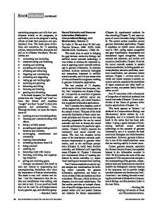
The initial choice for the weights was made randomly. The training procedure was repeated many times with different initial weight values. No significant differences, either in terms of the number of iterations or the error rate, were noticed due to initial weight selection. In all of the cases, stable classification performance was attained within 40 iterations.The best classification performance was obtained for an (Y value of 2.0. Next, a number of classification experiments were performed to gauge the effectiveness of the entropy net. These experiments include entropy net training using the backpropagation program of the PDP software [27. In this case, the learning rate of 0.5 was found unsuitable in terms of the number of iterations and classification performance. However, using the learning rate of 0.1 resulted in stable performance with 40 iterations. Another entropy net mapping thedecision tree given in [I91 for the same problem was also realized and trained. Fig. 14 summarizes the classification performance of sev-

Entropy CART Enlropy BP

Fig. 12. Three basic functions to generate waveform data.

Entropy AMlG 1-NN

CART Tree

Thetraining dataset consistsof 300examplesthatwere used to design the tree. The same set of examples was then used to train the entropy net. The test data have 5000 vectors. Using the training vectors, the AMlG algorithm produced the decision tree of Fig. 13 for waveform classification. The

Fig. 13. Decisiontreeforthewaveform datausingtheAMlC algorithm.Thefirst number at each internal node represents a feature axis, and the second number corresponds to a threshold value on that axis.

two numbers within each internal node of the tree respectively represent the feature axis and the threshold value on that axis. There are only 8 features out of 21 features that are presented in the tree. This indicates that the tree has already acquired the ability to discriminate between the important and nonimportant features of the problem as far as the classification task is concerned. To determine the learning progress of the entropy net, it was decided to perform classification on the test data after every ten iterations of weight adjustment with the training data and use the error rate on the test data as a measure of learning. Both of the layers were trained simultaneously.

1612

AMlG Tree 0

0.05

0.1

0.15

0.2

0 . 2 5 0.3

Error Rate

Fig. 14. Error rate for different classifiers for the waveform

recognition problem. Entropy.BP represents the results when the entropy net for the AMlG tree was trained using backpropagation.

era1classifiersand theentropy net for differentcases. These classifiers include the decison tree of Fig. 13, the decision tree from [19], and a nearest neighbor classifier that uses the training set as its database. It i s seen that the entropy net, whether trained using the LMS rule or backpropagation, provides an improvement over the tree classifier performance because of the adaptability arising due to the use of sigmoid nonlinearity. In all three realizations of the entropy net, the performance i s either better than the nearest neighbor performance or it is almost the same. The relative performance levels attained by different classifiers are similar to other studies for different classification tasks [8]. The shorter training time for the entropy net using the L M S ruleor backpropagation alsoconfirmsthe findings of other researchers that matching the network structure to the problem leads to less training time [I], [8].

VI. SUMMARY

AND

CONCLUSIONS

A new neural networkdesign methodology has been presented in this paper. This methodology has been developed by exploiting the similarities between the hierarchical classifiers of the traditional pattern recognition literature and the multiple-layer neural networks. It has been shown that the decision trees can be restructured as three-layer neural networks, called entropy networks. The entropy network architecture has the advantage of relatively fewer neural connections, which i s an attractive feature from the VLSl fabrication point of view. Since it i s possible to automatically generate decison trees using data-driven procedures,

PROCEEDINGS OF THE IEEE, VOL. 78, NO. 10, OCTOBER 1990

L

the tree-to-layered-network mapping rules provide a systematic tool t o obtain layered network architecture. One very important property of the entropy network architecture i s that the problem of credit assignment does not exist for these networks as it i s automatically solved during the tree learning stage. The issues of incremental learning and generalization have been discussed, and the importance of soft nonlinearities has been stressed. Finally, a two-stage procedure has been given where the dominant aspects of the problem are learned during the treedevelopment phase and the generalization of the learned knowledge takes place via the entropy network training. The effectiveness of the proposed methodology has been shown through two examples. It needs to be mentioned that the tree-to-network mapping approach i s not without any flaws. Because of the use of a single feature at each node during the tree design, it i s possible in many cases, the EX-OR problem for one, t o end up with very large trees. One possible solution to avoid very large trees i s to apply the Hotelling or principal component transformation [28]t o the data first. In terms of the entropy network, it i s equivalent t o adding an extra representation stage giving rise to a network which can be appropriately called a hoteling-entropy net. Such networks are currently under study, along with a study on the limitations of partially connected networks in comparison to fully connected feedforward networks with respect to missing data and broken connections. ACKNOWLEDGMENT

I gratefully acknowledge the assistance of N. Ramesh, M. Otten, and G.Yu in running some experiments for me. I also thank Prof. A. Jain for many useful discussions. REFEREN cEs D. J. Burr, "Experiments on neural net recognition of spoken and written text," /E€€ Trans. Acoust, Speech, Signal Processing, vol. 36, pp. 1162-1168, July 1988. R. P. Lippmann, "An introduction to computing with neural nets," lEEEASSPMag., pp. 4-22, Apr. 1987. A. Wieland and R. Leighton, "Geometric analysis of neural network capabilities," in Proc. /E€€ Int. Conf. Neural Networks, Vol. ///, San Diego, CA, June1987, pp. 385-392. D. E. Rumelhart, C. E. Hinton, and R. J. Williams, "Learning internal representation by error propagation," in D. E. Rurnelhart and J. L. McClelland, Eds., Parallel Distributed Processing: Explorations in the Microstructure of Cognition. Vol. 7: Foundations. Cambridge, MA: M.I.T. Press, 1986. D. H. Ackley, G. E. Hinton, and T. J. Sejnowski, "A learning algorithm for Boltzmann machines," Cognitive Sci., vol. 9, pp. 147-169, 1985. R. Hecht-Nielsen, "Counterpropagation networks," Appl. Opt., vol. 26, pp. 4979-4984, Dec. 1987. B. Widrow, R. G. Winter, and R. A. Baxter, "Layered neural nets for pattern recognition," /€€E Trans. Acoust., Speech, Signal Processing, vol. 36, pp. 1109-1118, July 1988. W. Y. Huang and R. P. Lippmann, "Comparison between neural net and conventional classifers," in Proc. / € € E 7st lnt. Conf. Neural Networks, Vol. IV, San Diego, CA, June1987, pp. 485-493. L. N. Kanal, "Problem-solving models and search strategies for pattern recognition," / € E € Trans. Pattern Anal. Machine Intell., vol. PAMI-1, pp. 194-201, Apr. 1979.

H. J. Payne and W. S. Meisel, "An algorithm for constructing optimal binary decision trees," /€€E Trans. Cornput., vol. C-25, pp. 905-916, Sept. 1977.

SETHI: ENTROPY NETS

[ l l ] L. A. Akers, M. R. Walker, D. K. Ferry, and R. 0. Grodin,"Lim-

121

131 141 151

161

171 181

ited interconnectivity in synthetic neural systems," in R. Eckmiller and C. v.d. Malsburg, Eds., Neural Computers. New York: Springer-Verlag, 1988. C. R. P. Hartmann, P. K. Varshney, K. C. Mehrotra, and C . L. Cerberich, "Application of information theory to the construction of efficient decision trees," /€€€ Trans. Inform. Theory, vOI. IT-28, pp. 565-577, July 1982. I. K. Sethi and B. Chaterjee,"Efficient decision treedesign for discrete variable pattern recognition problems," PatternRecognition, vol. 9, pp. 197-206, 1978. -, "A learning classifier scheme for discrete variable pattern recognition problems,'' /€€€ Trans. Syst., Man, Cybern., vol. SMC-8, pp. 49-52, Jan.1978. J. C. Stoffel, "A classifer design technique for discrete variable pattern recognition problems," I€€€Trans. Cornput., vol. C-23, pp. 428-441, 1974. E. G . Henrichon and K. S. Fu, "A nonparametric partitioning procedure for pattern classification," / € € E Trans. Comput., vol. C-18, pp. 614-624, July 1962. I. K. Sethi and G. P. R. Sarvarayudu, "Hierarchical classifier design using mutual information," I€€€ Trans. Pattern Anal. Machine Intell., vol. PAMI-4, pp. 441-445, July 1982. J.L. Talmon, "A multiclass nonparametric partitioning algorithm," in E. S. Celsema and L. N. Kanal, Eds., Pattern Recognition in Practice I / . Amsterdam: Elsevier Science Pub. B. V. (North-Holland). 1986. L. Breiman, J. Friedman, R. Olshen, and C. J. Stone, ClassificationandRegressionTrees. Belmont, CA: Wadsworth Int. Group, 1984. L. Hyafil and R. L. Rivest, "Constructing optimal binary decision trees is NP-complete," Inform. Processing Lett., vol. 5, pp. 15-17,1976. R. M. Fano, Transmission of Information. New York: Wiley, 1963. R. M. Goodman and P. Smyth, "Decision tree design from a

communication theory standpoint," /E€€ Trans. Inform. Theory, vol. 34, pp. 979-994, Sept. 1988. J. R. Quinlan, "Induction of decision trees," Machine Learning, vol. 1, pp. 81-106, 1986. T. Kohonen, Self-organization and Associative Memory. Berlin: Springer-Verlag, 1984. C. J. MatheusandW. E. Hohensee,"Learning inartifical neural systems," Univ. of Illnois, Urbana,Tech. Rep.TR-87-1394,1987. B. Widrow and M. E. Hoff, "Adaptive switching circuits," in 7960 IRE WESCON Conv. Rec., part 4, 1960, pp. 96-104. J.L. McClelland and D. E. Rumelhart, Explorationsin Parallel Distributed Processing. Cambridge, MA: M.I.T. Press, 1988. R. 0. Duda and P. E. Hart, Pattern Classification and Scene Analysis. New York: Wiley, 1973.

lshwar K. Sethi (Senior Member, IEEE)

received the B.Tech (Hons.), M. Tech., and Ph.D. degrees in Electronics and Electrical Communication Engineering from the Indian Institute of Technology, Kharagpur, India, in 1969, 1971, and 1977 respectively. He is presently an Associate Professorof Computer Science at Wayne State University, Detroit, Michigan. His current research interestsare in the applications of artificial neural networks to solve computer vision and pattern recognition problems. Prior to joining Wayne State University, he was on the faculty at the Indian Institute of Technology, Kharagpur, India. During the latter half of 1988, he was a Visiting Professoratthe Indian InstituteofTechnology, New Delhi, India. Dr. Sethi i s a member of the Association for Computing Machinery, the International Neural Network Society, and the International Society for Optical Engineering. He i s currently an Associate Editor of Pattern Recognition.

1613