Fully Convolutional Networks for Semantic Segmentation - arXiv [PDF]

1

Fully Convolutional Networks for Semantic Segmentation

arXiv:1605.06211v1 [cs.CV] 20 May 2016

Evan Shelhamer∗ , Jonathan Long∗ , and Trevor Darrell, Member, IEEE Abstract—Convolutional networks are powerful visual models that yield hierarchies of features. We show that convolutional networks by themselves, trained end-to-end, pixels-to-pixels, improve on the previous best result in semantic segmentation. Our key insight is to build “fully convolutional” networks that take input of arbitrary size and produce correspondingly-sized output with efficient inference and learning. We define and detail the space of fully convolutional networks, explain their application to spatially dense prediction tasks, and draw connections to prior models. We adapt contemporary classification networks (AlexNet, the VGG net, and GoogLeNet) into fully convolutional networks and transfer their learned representations by fine-tuning to the segmentation task. We then define a skip architecture that combines semantic information from a deep, coarse layer with appearance information from a shallow, fine layer to produce accurate and detailed segmentations. Our fully convolutional network achieves improved segmentation of PASCAL VOC (30% relative improvement to 67.2% mean IU on 2012), NYUDv2, SIFT Flow, and PASCAL-Context, while inference takes one tenth of a second for a typical image. Index Terms—Semantic Segmentation, Convolutional Networks, Deep Learning, Transfer Learning

F

1

I NTRODUCTION

C

ONVOLUTIONAL networks are driving advances in recognition. Convnets are not only improving for whole-image classification [1], [2], [3], but also making progress on local tasks with structured output. These include advances in bounding box object detection [4], [5], [6], part and keypoint prediction [7], [8], and local correspondence [8], [9]. The natural next step in the progression from coarse to fine inference is to make a prediction at every pixel. Prior approaches have used convnets for semantic segmentation [10], [11], [12], [13], [14], [15], [16], in which each pixel is labeled with the class of its enclosing object or region, but with shortcomings that this work addresses. We show that fully convolutional networks (FCNs) trained end-to-end, pixels-to-pixels on semantic segmentation exceed the previous best results without further machinery. To our knowledge, this is the first work to train FCNs end-to-end (1) for pixelwise prediction and (2) from supervised pre-training. Fully convolutional versions of existing networks predict dense outputs from arbitrarysized inputs. Both learning and inference are performed whole-image-at-a-time by dense feedforward computation and backpropagation. In-network upsampling layers enable pixelwise prediction and learning in nets with subsampling. This method is efficient, both asymptotically and absolutely, and precludes the need for the complications in other works. Patchwise training is common [10], [11], [12], [13], [16], but lacks the efficiency of fully convolutional training. Our approach does not make use of pre- and postprocessing complications, including superpixels [12], [14], proposals [14], [15], or post-hoc refinement by random fields ∗ Authors

•

contributed equally

E. Shelhamer, J. Long, and T. Darrell are with the Department of Electrical Engineering and Computer Science (CS Division), UC Berkeley. E-mail: {shelhamer,jonlong,trevor}@cs.berkeley.edu.

or local classifiers [12], [14]. Our model transfers recent success in classification [1], [2], [3] to dense prediction by reinterpreting classification nets as fully convolutional and fine-tuning from their learned representations. In contrast, previous works have applied small convnets without supervised pre-training [10], [12], [13]. Semantic segmentation faces an inherent tension between semantics and location: global information resolves what while local information resolves where. What can be done to navigate this spectrum from location to semantics? How can local decisions respect global structure? It is not immediately clear that deep networks for image classification yield representations sufficient for accurate, pixelwise recognition. In the conference version of this paper [17], we cast pre-trained networks into fully convolutional form, and augment them with a skip architecture that takes advantage of the full feature spectrum. The skip architecture fuses the feature hierarchy to combine deep, coarse, semantic information and shallow, fine, appearance information (see Section 4.3 and Figure 3). In this light, deep feature hierarchies encode location and semantics in a nonlinear local-toglobal pyramid. This journal paper extends our earlier work [17] through further tuning, analysis, and more results. Alternative choices, ablations, and implementation details better cover the space of FCNs. Tuning optimization leads to more accurate networks and a means to learn skip architectures all-atonce instead of in stages. Experiments that mask foreground and background investigate the role of context and shape. Results on the object and scene labeling of PASCAL-Context reinforce merging object segmentation and scene parsing as unified pixelwise prediction. In the next section, we review related work on deep classification nets, FCNs, recent approaches to semantic segmentation using convnets, and extensions to FCNs. The fol-

2 forward/inference backward/learning

6 25

. ion g.t ict ion ed t r a p nt is e me elw eg s x i p

96 96 21 4 4 6 40 40 38 38 25

96

21

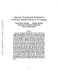
Fig. 1. Fully convolutional networks can efficiently learn to make dense predictions for per-pixel tasks like semantic segmentation.

lowing sections explain FCN design, introduce our architecture with in-network upsampling and skip layers, and describe our experimental framework. Next, we demonstrate improved accuracy on PASCAL VOC 2011-2, NYUDv2, SIFT Flow, and PASCAL-Context. Finally, we analyze design choices, examine what cues can be learned by an FCN, and calculate recognition bounds for semantic segmentation.

2

R ELATED W ORK

Our approach draws on recent successes of deep nets for image classification [1], [2], [3] and transfer learning [18], [19]. Transfer was first demonstrated on various visual recognition tasks [18], [19], then on detection, and on both instance and semantic segmentation in hybrid proposalclassifier models [5], [14], [15]. We now re-architect and fine-tune classification nets to direct, dense prediction of semantic segmentation. We chart the space of FCNs and relate prior models both historical and recent. Fully convolutional networks To our knowledge, the idea of extending a convnet to arbitrary-sized inputs first appeared in Matan et al. [20], which extended the classic LeNet [21] to recognize strings of digits. Because their net was limited to one-dimensional input strings, Matan et al. used Viterbi decoding to obtain their outputs. Wolf and Platt [22] expand convnet outputs to 2-dimensional maps of detection scores for the four corners of postal address blocks. Both of these historical works do inference and learning fully convolutionally for detection. Ning et al. [10] define a convnet for coarse multiclass segmentation of C. elegans tissues with fully convolutional inference. Fully convolutional computation has also been exploited in the present era of many-layered nets. Sliding window detection by Sermanet et al. [4], semantic segmentation by Pinheiro and Collobert [13], and image restoration by Eigen et al. [23] do fully convolutional inference. Fully convolutional training is rare, but used effectively by Tompson et al. [24] to learn an end-to-end part detector and spatial model for pose estimation, although they do not exposit on or analyze this method. Dense prediction with convnets Several recent works have applied convnets to dense prediction problems, including semantic segmentation by Ning et al. [10], Farabet et al. [12], and Pinheiro and Collobert [13]; boundary prediction for electron microscopy by Ciresan et al. [11] and for natural images by a hybrid convnet/nearest neighbor model by

Ganin and Lempitsky [16]; and image restoration and depth estimation by Eigen et al. [23], [25]. Common elements of these approaches include • small models restricting capacity and receptive fields; • patchwise training [10], [11], [12], [13], [16]; • refinement by superpixel projection, random field regularization, filtering, or local classification [11], [12], [16]; • “interlacing” to obtain dense output [4], [13], [16]; • multi-scale pyramid processing [12], [13], [16]; • saturating tanh nonlinearities [12], [13], [23]; and • ensembles [11], [16], whereas our method does without this machinery. However, we do study patchwise training (Section 3.4) and “shift-andstitch” dense output (Section 3.2) from the perspective of FCNs. We also discuss in-network upsampling (Section 3.3), of which the fully connected prediction by Eigen et al. [25] is a special case. Unlike these existing methods, we adapt and extend deep classification architectures, using image classification as supervised pre-training, and fine-tune fully convolutionally to learn simply and efficiently from whole image inputs and whole image ground thruths. Hariharan et al. [14] and Gupta et al. [15] likewise adapt deep classification nets to semantic segmentation, but do so in hybrid proposal-classifier models. These approaches finetune an R-CNN system [5] by sampling bounding boxes and/or region proposals for detection, semantic segmentation, and instance segmentation. Neither method is learned end-to-end. They achieve the previous best segmentation results on PASCAL VOC and NYUDv2 respectively, so we directly compare our standalone, end-to-end FCN to their semantic segmentation results in Section 5. Combining feature hierarchies We fuse features across layers to define a nonlinear local-to-global representation that we tune end-to-end. The Laplacian pyramid [26] is a classic multi-scale representation made of fixed smoothing and differencing. The jet of Koenderink and van Doorn [27] is a rich, local feature defined by compositions of partial derivatives. In the context of deep networks, Sermanet et al. [28] fuse intermediate layers but discard resolution in doing so. In contemporary work Hariharan et al. [29] and Mostajabi et al. [30] also fuse multiple layers but do not learn end-to-end and rely on fixed bottom-up grouping. FCN extensions Following the conference version of this paper [17], FCNs have been extended to new tasks and data. Tasks include region proposals [31], contour detection [32], depth regression [33], optical flow [34], and weaklysupervised semantic segmentation [35], [36], [37], [38]. In addition, new works have improved the FCNs presented here to further advance the state-of-the-art in semantic segmentation. The DeepLab models [39] raise output resolution by dilated convolution and dense CRF inference. The joint CRFasRNN [40] model is an end-to-end integration of the CRF for further improvement. ParseNet [41] normalizes features for fusion and captures context with global pooling. The “deconvolutional network” approach of [42] restores resolution by proposals, stacks of learned deconvolution, and unpooling. U-Net [43] combines skip layers and learned deconvolution for pixel labeling of microscopy images. The dilation architecture of [44] makes

3

thorough use of dilated convolution for pixel-precise output without a random field or skip layers.

3

F ULLY C ONVOLUTIONAL N ETWORKS

Each layer output in a convnet is a three-dimensional array of size h × w × d, where h and w are spatial dimensions, and d is the feature or channel dimension. The first layer is the image, with pixel size h × w, and d channels. Locations in higher layers correspond to the locations in the image they are path-connected to, which are called their receptive fields. Convnets are inherently translation invariant. Their basic components (convolution, pooling, and activation functions) operate on local input regions, and depend only on relative spatial coordinates. Writing xij for the data vector at location (i, j) in a particular layer, and yij for the following layer, these functions compute outputs yij by

yij = fks ({xsi+δi,sj+δj }0≤δi,δj 0.2 according to the numbers in Section 3.1). Figure 5 shows the effect of this form of sampling on convergence. We find that sampling does not have a significant effect on convergence rate compared to whole image training, but takes significantly more time due to the larger number of images that need to be considered per batch. We therefore choose unsampled, whole image training in our other experiments. Class balancing Fully convolutional training can balance classes by weighting or sampling the loss. Although our labels are mildly unbalanced (about 3/4 are background), we find class balancing unnecessary. Dense Prediction The scores are upsampled to the input dimensions by backward convolution layers within the net. Final layer backward convolution weights are fixed to bilinear interpolation, while intermediate upsampling layers are initialized to bilinear interpolation, and then learned. This simple, end-to-end method is accurate and fast. Augmentation We tried augmenting the training data by randomly mirroring and “jittering” the images by translating them up to 32 pixels (the coarsest scale of prediction) in each direction. This yielded no noticeable improvement. Implementation All models are trained and tested with Caffe [54] on a single NVIDIA Titan X. Our models and code are publicly available at http://fcn.berkeleyvision.org.

8

5

R ESULTS

We test our FCN on semantic segmentation and scene parsing, exploring PASCAL VOC, NYUDv2, SIFT Flow, and PASCAL-Context. Although these tasks have historically distinguished between objects and regions, we treat both uniformly as pixel prediction. We evaluate our FCN skip architecture on each of these datasets, and then extend it to multi-modal input for NYUDv2 and multi-task prediction for the semantic and geometric labels of SIFT Flow. All experiments follow the same network architecture and optimization settings decided on in Section 4. Metrics We report metrics from common semantic segmentation and scene parsing evaluations that are variations on pixel accuracy and region intersection over union (IU): P P • pixel accuracy: i nii / i ti P • mean accuraccy: (1/ncl ) i nii /ti   P P • mean IU: (1/ncl ) i nii / ti + j nji − nii −1

  P i ti nii / ti + j nji − nii

• frequency weighted IU: ( k tk ) where nij is the number of pixels of class i predicted to belong to class j , there are ncl different classes, and ti = P j nij is the total number of pixels of class i. PASCAL VOC Table 4 gives the performance of our FCN-8s on the test sets of PASCAL VOC 2011 and 2012, and compares it to the previous best, SDS [14], and the wellknown R-CNN [5]. We achieve the best results on mean IU by 30% relative. Inference time is reduced 114× (convnet only, ignoring proposals and refinement) or 286× (overall). NYUDv2 [55] is an RGB-D dataset collected using the Microsoft Kinect. It has 1,449 RGB-D images, with pixelwise labels that have been coalesced into a 40 class semantic segmentation task by Gupta et al. [56]. We report results on the standard split of 795 training images and 654 testing images. Table 5 gives the performance of several net variations. First we train our unmodified coarse model (FCN-32s) on RGB images. To add depth information, we train on a model upgraded to take four-channel RGB-D input (early fusion). This provides little benefit, perhaps due to similar number of parameters or the difficulty of propagating meaningful gradients all the way through the net. Following the success of Gupta et al. [15], we try the three-dimensional HHA encoding of depth and train a net on just this information. To effectively combine color and depth, we define a “late fusion” of RGB and HHA that averages the final layer scores from both nets and learn the resulting two-stream net endto-end. This late fusion RGB-HHA net is the most accurate. SIFT Flow is a dataset of 2,688 images with pixel labels for 33 semantic classes (“bridge”, “mountain”, “sun”), as well as three geometric classes (“horizontal”, “vertical”, and “sky”). An FCN can naturally learn a joint representation that simultaneously predicts both types of labels. We learn a two-headed version of FCN-32/16/8s with semantic and geometric prediction layers and losses. This net performs as well on both tasks as two independently trained nets, while learning and inference are essentially as fast as each independent net by itself. The results in Table 6, computed on the standard split into 2,488 training and 200 test images,6 show better performance on both tasks.

P

TABLE 4 Our FCN gives a 30% relative improvement on the previous best PASCAL VOC 11/12 test results with faster inference and learning. mean IU VOC2011 test

mean IU VOC2012 test

inference time

47.9 52.6 67.5

51.6 67.2

∼ 50 s ∼ 100 ms

R-CNN [5] SDS [14] FCN-8s

TABLE 5 Results on NYUDv2. RGB-D is early-fusion of the RGB and depth channels at the input. HHA is the depth embedding of [15] as horizontal disparity, height above ground, and the angle of the local surface normal with the inferred gravity direction. RGB-HHA is the jointly trained late fusion model that sums RGB and HHA predictions.

P

6. Three of the SIFT Flow classes are not present in the test set. We made predictions across all 33 classes, but only included classes actually present in the test set in our evaluation.

Gupta et al. [15] FCN-32s RGB FCN-32s RGB-D FCN-32s HHA FCN-32s RGB-HHA

pixel acc.

mean mean f.w. acc. IU IU

60.3 61.8 62.1 58.3 65.3

44.7 44.8 35.7 44.0

28.6 31.6 31.7 25.2 33.3

47.0 46.0 46.3 41.7 48.6

TABLE 6 Results on SIFT Flow6 with semantics (center) and geometry (right). Farabet is a multi-scale convnet trained on class-balanced or natural frequency samples. Pinheiro is the multi-scale, recurrent convnet R CNN3 (◦3 ). The metric for geometry is pixel accuracy.

Liu et al. [57] Tighe et al. [58] transfer Tighe et al. [59] SVM Tighe et al. [59] SVM+MRF Farabet et al. [12] natural Farabet et al. [12] balanced Pinheiro et al. [13] FCN-8s

pixel acc.

mean mean f.w. acc. IU IU

76.7 75.6 78.6 72.3 78.5 77.7 85.9

41.1 39.2 50.8 29.6 29.8 53.9

41.2

77.2

geom. acc. 90.8 94.6

TABLE 7 Results on PASCAL-Context for the 59 class task. CFM is convolutional feature masking [60] and segment pursuit with the VGG net. O2 P is the second order pooling method [61] as reported in the errata of [62].

59 class

pixel acc.

mean mean f.w. acc. IU IU

O2 P CFM FCN-32s FCN-16s FCN-8s

65.5 66.9 67.5

49.1 51.3 52.3

18.1 34.4 36.7 38.4 39.1

50.9 52.3 53.0

PASCAL-Context [62] provides whole scene annotations of PASCAL VOC 2010. While there are 400+ classes, we follow the 59 class task defined by [62] that picks the most frequent classes. We train and evaluate on the training and val sets respectively. In Table 7 we compare to the previous best result on this task. FCN-8s scores 39.1 mean IU for a relative improvement of more than 10%.

9

FCN-8s

SDS [14]

Ground Truth

Image

TABLE 8 The role of foreground, background, and shape cues. All scores are the mean intersection over union metric excluding background. The architecture and optimization are fixed to those of FCN-32s (Reference) and only input masking differs. train

Reference Reference-FG Reference-BG FG-only BG-only Shape

Fig. 6. Fully convolutional networks improve performance on PASCAL. The left column shows the output of our most accurate net, FCN-8s. The second shows the output of the previous best method by Hariharan et al. [14]. Notice the fine structures recovered (first row), ability to separate closely interacting objects (second row), and robustness to occluders (third row). The fifth and sixth rows show failure cases: the net sees lifejackets in a boat as people and confuses human hair with a dog.

6

A NALYSIS

We examine the learning and inference of fully convolutional networks. Masking experiments investigate the role of context and shape by reducing the input to only foreground, only background, or shape alone. Defining a “null” background model checks the necessity of learning a background classifier for semantic segmentation. We detail an approximation between momentum and batch size to further tune whole image learning. Finally, we measure bounds on task accuracy for given output resolutions to show there is still much to improve. 6.1

Cues

Given the large receptive field size of an FCN, it is natural to wonder about the relative importance of foreground and background pixels in the prediction. Is foreground appearance sufficient for inference, or does the context influence the output? Conversely, can a network learn to recognize a class by its shape and context alone? Masking To explore these issues we experiment with masked versions of the standard PASCAL VOC segmentation challenge. We both mask input to networks trained on normal PASCAL, and learn new networks on the masked PASCAL. See Table 8 for masked results.

test

FG

BG

FG

BG

mean IU

keep keep keep keep mask mask

keep keep keep mask keep mask

keep keep mask keep mask mask

keep mask keep mask keep mask

84.8 81.0 19.8 76.1 37.8 29.1

Masking the foreground at inference time is catastrophic. However, masking the foreground during learning yields a network capable of recognizing object segments without observing a single pixel of the labeled class. Masking the background has little effect overall but does lead to class confusion in certain cases. When the background is masked during both learning and inference, the network unsurprisingly achieves nearly perfect background accuracy; however certain classes are more confused. All-in-all this suggests that FCNs do incorporate context even though decisions are driven by foreground pixels. To separate the contribution of shape, we learn a net restricted to the simple input of foreground/background masks. The accuracy in this shape-only condition is lower than when only the foreground is masked, suggesting that the net is capable of learning context to boost recognition. Nonetheless, it is surprisingly accurate. See Figure 7. Background modeling It is standard in detection and semantic segmentation to have a background model. This model usually takes the same form as the models for the classes of interest, but is supervised by negative instances. In our experiments we have followed the same approach, learning parameters to score all classes including background. Is this actually necessary, or do class models suffice? To investigate, we define a net with a “null” background model that gives a constant score of zero. Instead of training with the softmax loss, which induces competition by normalizing across classes, we train with the sigmoid crossentropy loss, which independently normalizes each score. For inference each pixel is assigned the highest scoring class. In all other respects the experiment is identical to our FCN32s on PASCAL VOC. The null background net scores 1 point lower than the reference FCN-32s and a control FCN32s trained on all classes including background with the sigmoid cross-entropy loss. To put this drop in perspective, note that discarding the background model in this way reduces the total number of parameters by less than 0.1%. Nonetheless, this result suggests that learning a dedicated background model for semantic segmentation is not vital. 6.2 Momentum and batch size In comparing optimization schemes for FCNs, we find that “heavy” online learning with high momentum trains more accurate models in less wall clock time (see Section 4.2). Here we detail a relationship between momentum and batch size that motivates heavy learning.

10

Image

Ground Truth

Output

Input

learning. In practice, we find that online learning works well and yields better FCN models in less wall clock time.

6.3

Upper bounds on IU

FCNs achieve good performance on the mean IU segmentation metric even with spatially coarse semantic prediction. To better understand this metric and the limits of this approach with respect to it, we compute approximate upper bounds on performance with prediction at various resolutions. We do this by downsampling ground truth images and then upsampling back to simulate the best results obtainable with a particular downsampling factor. The following table gives the mean IU on a subset5 of PASCAL 2011 val for various downsampling factors. factor

mean IU

128 64 32 16 8 4

50.9 73.3 86.1 92.8 96.4 98.5

Fig. 7. FCNs learn to recognize by shape when deprived of other input detail. From left to right: regular image (not seen by network), ground truth, output, mask input.

Pixel-perfect prediction is clearly not necessary to achieve mean IU well above state-of-the-art, and, conversely, mean IU is a not a good measure of fine-scale accuracy. The gaps between oracle and state-of-the-art accuracy at every stride suggest that recognition and not resolution is the bottleneck for this metric.

By writing the updates computed by gradient accumulation as a non-recursive sum, we will see that momentum and batch size can be approximately traded off, which suggests alternative training parameters. Let gt be the step taken by minibatch SGD with momentum at time t,

7

gt = −η

k−1 X

∇θ `(xkt+i ; θt−1 ) + pgt−1 ,

i=0

where `(x; θ) is the loss for example x and parameters θ, p < 1 is the momentum, k is the batch size, and η is the learning rate. Expanding this recurrence as an infinite sum with geometric coefficients, we have

gt = −η

∞ k−1 X X

ps ∇θ `(xk(t−s)+i ; θt−s ).

C ONCLUSION

Fully convolutional networks are a rich class of models that address many pixelwise tasks. FCNs for semantic segmentation dramatically improve accuracy by transferring pretrained classifier weights, fusing different layer representations, and learning end-to-end on whole images. End-toend, pixel-to-pixel operation simultaneously simplifies and speeds up learning and inference. All code for this paper is open source in Caffe, and all models are freely available in the Caffe Model Zoo. Further works have demonstrated the generality of fully convolutional networks for a variety of image-to-image tasks.

s=0 i=0

In other words, each example is included in the sum with coefficient pbj/kc , where the index j orders the examples from most recently considered to least recently considered. Approximating this expression by dropping the floor, we see that learning with momentum p and batch size k appears to be similar to learning with momentum p0 and batch 0 size k 0 if p(1/k) = p0(1/k ) . Note that this is not an exact equivalence: a smaller batch size results in more frequent weight updates, and may make more learning progress for the same number of gradient computations. For typical FCN values of momentum 0.9 and a batch size of 20 images, an approximately equivalent training regime uses momentum 0.9(1/20) ≈ 0.99 and a batch size of one, resulting in online

ACKNOWLEDGEMENTS This work was supported in part by DARPA’s MSEE and SMISC programs, NSF awards IIS-1427425, IIS-1212798, IIS1116411, and the NSF GRFP, Toyota, and the Berkeley Vision and Learning Center. We gratefully acknowledge NVIDIA for GPU donation. We thank Bharath Hariharan and Saurabh Gupta for their advice and dataset tools. We thank Sergio Guadarrama for reproducing GoogLeNet in Caffe. We thank Jitendra Malik for his helpful comments. Thanks to Wei Liu for pointing out an issue wth our SIFT Flow mean IU computation and an error in our frequency weighted mean IU formula.

11

R EFERENCES [1] [2] [3] [4] [5] [6] [7] [8] [9] [10]

[11] [12] [13] [14] [15] [16] [17] [18] [19] [20] [21] [22] [23] [24] [25] [26] [27]

A. Krizhevsky, I. Sutskever, and G. E. Hinton, “Imagenet classification with deep convolutional neural networks.” in NIPS, 2012. 1, 2, 3, 5 K. Simonyan and A. Zisserman, “Very deep convolutional networks for large-scale image recognition,” in ICLR, 2015. 1, 2, 3, 5 C. Szegedy, W. Liu, Y. Jia, P. Sermanet, S. Reed, D. Anguelov, D. Erhan, V. Vanhoucke, and A. Rabinovich, “Going deeper with convolutions,” in CVPR, 2015. 1, 2, 3, 5 P. Sermanet, D. Eigen, X. Zhang, M. Mathieu, R. Fergus, and Y. LeCun, “OverFeat: Integrated recognition, localization and detection using convolutional networks,” in ICLR, 2014. 1, 2, 4 R. Girshick, J. Donahue, T. Darrell, and J. Malik, “Region-based convolutional networks for accurate object detection and segmentation,” PAMI, 2015. 1, 2, 8 K. He, X. Zhang, S. Ren, and J. Sun, “Spatial pyramid pooling in deep convolutional networks for visual recognition,” in ECCV, 2014. 1 N. Zhang, J. Donahue, R. Girshick, and T. Darrell, “Part-based R-CNNs for fine-grained category detection,” in ECCV, 2014, pp. 834–849. 1 J. Long, N. Zhang, and T. Darrell, “Do convnets learn correspondence?” in NIPS, 2014. 1 P. Fischer, A. Dosovitskiy, and T. Brox, “Descriptor matching with convolutional neural networks: a comparison to SIFT,” arXiv preprint arXiv:1405.5769, 2014. 1 F. Ning, D. Delhomme, Y. LeCun, F. Piano, L. Bottou, and P. E. Barbano, “Toward automatic phenotyping of developing embryos from videos,” Image Processing, IEEE Transactions on, vol. 14, no. 9, pp. 1360–1371, 2005. 1, 2, 4, 7 D. C. Ciresan, A. Giusti, L. M. Gambardella, and J. Schmidhuber, “Deep neural networks segment neuronal membranes in electron microscopy images.” in NIPS, 2012, pp. 2852–2860. 1, 2, 4, 7 C. Farabet, C. Couprie, L. Najman, and Y. LeCun, “Learning hierarchical features for scene labeling,” PAMI, 2013. 1, 2, 4, 7, 8 P. H. Pinheiro and R. Collobert, “Recurrent convolutional neural networks for scene labeling,” in ICML, 2014. 1, 2, 4, 7, 8 B. Hariharan, P. Arbel´aez, R. Girshick, and J. Malik, “Simultaneous detection and segmentation,” in ECCV, 2014. 1, 2, 4, 5, 7, 8, 9 S. Gupta, R. Girshick, P. Arbelaez, and J. Malik, “Learning rich features from RGB-D images for object detection and segmentation,” in ECCV, 2014. 1, 2, 8 Y. Ganin and V. Lempitsky, “N4 -fields: Neural network nearest neighbor fields for image transforms,” in ACCV, 2014. 1, 2, 7 J. Long, E. Shelhamer, and T. Darrell, “Fully convolutional networks for semantic segmentation,” CVPR, 2015. 1, 2 J. Donahue, Y. Jia, O. Vinyals, J. Hoffman, N. Zhang, E. Tzeng, and T. Darrell, “DeCAF: A deep convolutional activation feature for generic visual recognition,” in ICML, 2014. 2 M. D. Zeiler and R. Fergus, “Visualizing and understanding convolutional networks,” in ECCV, 2014, pp. 818–833. 2, 4 O. Matan, C. J. Burges, Y. LeCun, and J. S. Denker, “Multi-digit recognition using a space displacement neural network,” in NIPS, 1991, pp. 488–495. 2 Y. LeCun, B. Boser, J. Denker, D. Henderson, R. E. Howard, W. Hubbard, and L. D. Jackel, “Backpropagation applied to handwritten zip code recognition,” in Neural Computation, 1989. 2, 3 R. Wolf and J. C. Platt, “Postal address block location using a convolutional locator network,” in NIPS, 1994, pp. 745–745. 2 D. Eigen, D. Krishnan, and R. Fergus, “Restoring an image taken through a window covered with dirt or rain,” in ICCV, 2013, pp. 633–640. 2 J. Tompson, A. Jain, Y. LeCun, and C. Bregler, “Joint training of a convolutional network and a graphical model for human pose estimation,” in NIPS, 2014. 2 D. Eigen, C. Puhrsch, and R. Fergus, “Depth map prediction from a single image using a multi-scale deep network,” in NIPS, 2014. 2 P. Burt and E. Adelson, “The laplacian pyramid as a compact image code,” Communications, IEEE Transactions on, vol. 31, no. 4, pp. 532–540, 1983. 2, 6 J. J. Koenderink and A. J. van Doorn, “Representation of local geometry in the visual system,” Biological cybernetics, vol. 55, no. 6, pp. 367–375, 1987. 2, 6

[28] P. Sermanet, K. Kavukcuoglu, S. Chintala, and Y. LeCun, “Pedestrian detection with unsupervised multi-stage feature learning,” in CVPR, 2013. 2 [29] B. Hariharan, P. Arbel´aez, R. Girshick, and J. Malik, “Hypercolumns for object segmentation and fine-grained localization,” in CVPR, 2015. 2 [30] M. Mostajabi, P. Yadollahpour, and G. Shakhnarovich, “Feedforward semantic segmentation with zoom-out features,” in CVPR, 2015. 2 [31] S. Ren, K. He, R. Girshick, and J. Sun, “Faster R-CNN: Towards real-time object detection with region proposal networks,” in NIPS, 2015. 2 [32] S. Xie and Z. Tu, “Holistically-nested edge detection,” in ICCV, 2015. 2 [33] F. Liu, C. Shen, G. Lin, and I. Reid, “Learning depth from single monocular images using deep convolutional neural fields,” PAMI, 2015. 2 [34] P. Fischer, A. Dosovitskiy, E. Ilg, P. Husser, C. Hazrba, V. Golkov, P. van der Smagt, D. Cremers, and T. Brox, “Learning optical flow with convolutional networks,” in ICCV, 2015. 2 ¨ [35] D. Pathak, P. Kr¨ahenbuhl, and T. Darrell, “Constrained convolutional neural networks for weakly supervised segmentation,” in ICCV, 2015. 2 [36] G. Papandreou, L.-C. Chen, K. Murphy, and A. L. Yuille, “Weaklyand semi-supervised learning of a DCNN for semantic image segmentation,” in ICCV, 2015. 2 [37] J. Dai, K. He, and J. Sun, “Boxsup: Exploiting bounding boxes to supervise convolutional networks for semantic segmentation,” in ICCV, 2015. 2 [38] S. Hong, H. Noh, and B. Han, “Decoupled deep neural network for semi-supervised semantic segmentation,” in NIPS, 2015, pp. 1495–1503. 2 [39] L.-C. Chen, G. Papandreou, I. Kokkinos, K. Murphy, and A. L. Yuille, “Semantic image segmentation with deep convolutional nets and fully connected CRFs,” in ICLR, 2015. 2 [40] S. Zheng, S. Jayasumana, B. Romera-Paredes, V. Vineet, Z. Su, D. Du, C. Huang, and P. Torr, “Conditional random fields as recurrent neural networks,” in ICCV, 2015. 2 [41] W. Liu, A. Rabinovich, and A. C. Berg, “ParseNet: Looking wider to see better,” arXiv preprint arXiv:1506.04579, 2015. 2 [42] H. Noh, S. Hong, and B. Han, “Learning deconvolution network for semantic segmentation,” in ICCV, 2015. 2 [43] O. Ronneberger, P. Fischer, and T. Brox, “U-Net: Convolutional networks for biomedical image segmentation,” in MICCAI, 2015. 2 [44] F. Yu and V. Koltun, “Multi-scale context aggregation by dilated convolutions,” in ICLR, 2016. 2, 4 [45] A. Giusti, D. C. Cires¸an, J. Masci, L. M. Gambardella, and J. Schmidhuber, “Fast image scanning with deep max-pooling convolutional neural networks,” in ICIP, 2013. 3, 4 [46] M. Holschneider, R. Kronland-Martinet, J. Morlet, and P. Tchamitchian, “A real-time algorithm for signal analysis with the help of the wavelet transform,” pp. 286–297, 1989. 4 [47] S. Mallat, A wavelet tour of signal processing, 2nd ed. Academic press, 1999. 4 [48] P. P. Vaidyanathan, “Multirate digital filters, filter banks, polyphase networks, and applications: A tutorial,” Proceedings of the IEEE, vol. 78, no. 1, pp. 56–93, 1990. 4 [49] L. Wan, M. Zeiler, S. Zhang, Y. L. Cun, and R. Fergus, “Regularization of neural networks using dropconnect,” in ICML, 2013, pp. 1058–1066. 4 [50] M. Everingham, L. Van Gool, C. K. I. Williams, J. Winn, and A. Zisserman, “The PASCAL Visual Object Classes Challenge 2011 (VOC2011) Results,” http://www.pascalnetwork.org/challenges/VOC/voc2011/workshop/index.html. 4 [51] C. M. Bishop, Pattern recognition and machine learning. SpringerVerlag New York, 2006, p. 229. 5 [52] B. Hariharan, P. Arbelaez, L. Bourdev, S. Maji, and J. Malik, “Semantic contours from inverse detectors,” in ICCV, 2011. 7 ¨ [53] Y. A. LeCun, L. Bottou, G. B. Orr, and K.-R. Muller, “Efficient backprop,” in Neural networks: Tricks of the trade, 1998, pp. 9–48. 7 [54] Y. Jia, E. Shelhamer, J. Donahue, S. Karayev, J. Long, R. Girshick, S. Guadarrama, and T. Darrell, “Caffe: Convolutional architecture for fast feature embedding,” arXiv preprint arXiv:1408.5093, 2014. 7

12

[55] N. Silberman, D. Hoiem, P. Kohli, and R. Fergus, “Indoor segmentation and support inference from RGBD images,” in ECCV, 2012. 8 [56] S. Gupta, P. Arbelaez, and J. Malik, “Perceptual organization and recognition of indoor scenes from RGB-D images,” in CVPR, 2013. 8 [57] C. Liu, J. Yuen, and A. Torralba, “Sift flow: Dense correspondence across scenes and its applications,” PAMI, vol. 33, no. 5, pp. 978– 994, 2011. 8 [58] J. Tighe and S. Lazebnik, “Superparsing: scalable nonparametric image parsing with superpixels,” in ECCV, 2010, pp. 352–365. 8 [59] ——, “Finding things: Image parsing with regions and perexemplar detectors,” in CVPR, 2013. 8 [60] J. Dai, K. He, and J. Sun, “Convolutional feature masking for joint object and stuff segmentation,” in CVPR, 2015. 8 [61] J. Carreira, R. Caseiro, J. Batista, and C. Sminchisescu, “Semantic segmentation with second-order pooling,” in ECCV, 2012. 8 [62] R. Mottaghi, X. Chen, X. Liu, N.-G. Cho, S.-W. Lee, S. Fidler, R. Urtasun, and A. Yuille, “The role of context for object detection and semantic segmentation in the wild,” in CVPR, 2014, pp. 891– 898. 8