GAECH: Genetic Algorithm Based Energy Efficient Clustering ...

Hindawi Publishing Corporation Journal of Sensors Volume 2015, Article ID 715740, 8 pages http://dx.doi.org/10.1155/2015/715740

Research Article GAECH: Genetic Algorithm Based Energy Efficient Clustering Hierarchy in Wireless Sensor Networks B. Baranidharan and B. Santhi School of Computing, SASTRA University, Thanjavur, Tamil Nadu 613401, India Correspondence should be addressed to B. Baranidharan; [email protected] Received 10 June 2015; Revised 1 August 2015; Accepted 5 August 2015 Academic Editor: Fanli Meng Copyright © 2015 B. Baranidharan and B. Santhi. This is an open access article distributed under the Creative Commons Attribution License, which permits unrestricted use, distribution, and reproduction in any medium, provided the original work is properly cited. Clustering the Wireless Sensor Networks (WSNs) is the major issue which determines the lifetime of the network. The parameters chosen for clustering should be appropriate to form the clusters according to the need of the applications. Some of the well-known clustering techniques in WSN are designed only to reduce overall energy consumption in the network and increase the network lifetime. These algorithms achieve increased lifetime, but at the cost of overloading individual sensor nodes. Load balancing among the nodes in the network is also equally important in achieving increased lifetime. First Node Die (FND), Half Node Die (HND), and Last Node Die (LND) are the different metrics for analysing lifetime of the network. In this paper, a new clustering algorithm, Genetic Algorithm based Energy efficient Clustering Hierarchy (GAECH) algorithm, is proposed to increase FND, HND, and LND with a novel fitness function. The fitness function in GAECH forms well-balanced clusters considering the core parameters of a cluster, which again increases both the stability period and lifetime of the network. The experimental results also clearly indicate better performance of GAECH over other algorithms in all the necessary aspects.

1. Introduction The rapid development in microelectromechanical systems (MEMS) led to the development of miniature sensor nodes [1]. Wireless Sensor Network (WSN) is the interconnection of these small sensor nodes in large number. WSN plays a vital role in environmental monitoring, traffic monitoring, disaster prevention, and national border surveillance [1]. The individual sensor node generates data by sensing its surroundings and sends it to the central base station (BS). Each node is embedded with a battery and these batteries are mostly not rechargeable. The communication activities carried over in the sensor node will be consuming more energy than its sensing and computation activities [2]. If the battery power of one node gets drained, the node became useless and literally called dead node. All the sensor nodes are able to directly transmit their generated data to BS, but this leads to more energy consumption and affects the lifetime of the network [3]. To reduce the overall energy consumption of the network, the nearby nodes or the nodes having the same characteristics are grouped

together to form clusters. A cluster head (CH) will be elected among the nodes to manage the cluster activities. The responsibilities of the CHs are collecting the data from their member nodes, aggregating the collected data, and transmitting the aggregated data to BS. But the CH node will not be involved in sensing activities like other nodes. Compared with member nodes (non-CH), usually a CH node has to spend more energy because of its data reception, aggregation, and transmission to BS [4]. Various such clustering algorithms in WSN are discussed in detail in [5]. Earlier works like in [6, 7] concentrated more on efficient data gathering mechanism in WSN and not on clustering process. But later, the clustering mechanism occurs in the distributed way which proved to be more suitable for WSN [8]. As a further improvement, reducing the communication distance within the clustering framework had gained attention [9]. Reducing the intra- and intercluster communication in the clustering architecture gathered attention [10] along with distributed clustering approach. Instead of forming dynamic clusters, fixed grid structure is also used, but again it is another form of clustering architecture [11].

2 In most of the existing clustering algorithms, the overall energy consumption of the network is reduced, but it comes at the cost of uneven energy consumption among the sensor nodes. In certain cases, when we are trying to balance the energy spent among the nodes, the overall energy consumption may rise. Various computational intelligence techniques have been applied to increase the WSNs lifetime [12]. In order for a trade-off between overall energy consumption and energy balancing in the network, a new clustering algorithm, Genetic Algorithm based Energy efficient Clustering Hierarchy (GAECH), is proposed in this paper. Although many clustering algorithms using genetic approach [13, 14] are proposed, these protocols fail to increase the stability period of the network. The period till the First Node Die (FND) in the network is referred as stability period. FND is an important parameter in deciding the reliability of the network. GAECH achieves both increased lifetime and stability period of the WSN using enhanced fitness function. The paper is organized as follows. Section 2 makes a brief survey of some of the clustering algorithms with their pros and cons. Section 3 describes basic terminologies used in genetic algorithms. Section 4 discusses the proposed GAECH algorithm with its fitness parameters. Section 5 deals with the simulation setup environment for various clustering algorithms and Section 6 discusses the results of the experiments.

2. Related Work LEACH [15] was the pioneer clustering protocol in WSN. It forms clusters in a distributed manner. Setup and steady state are the two phases in LEACH. At first, in the setup phase, each node decides itself to be CH or not. This decision was influenced by various factors like number of times it elected as head, current round, and the percentage of allowed CHs in the network. Then, the CH elected nodes advertise it among the nodes. The other non-CH nodes join the nearby elected CH which is computed based on the received signal strength indicator (RSSI). Followed by this, TDMA schedule is created for the newly formed clusters by the respective heads. In steady state phase, data generated from the member nodes is forwarded to the CHs in its allotted time schedule. The probabilistic way of election of CHs leads to election of noneligible CHs which costs the overall lifetime of the network at the end. In the HEED [16] protocol, the remaining energy of the sensor nodes is the most important parameter for stochastic selection of CHs. Node degree or average distance to neighbours is used to conclude the CH when there is a tie between two sensor nodes. HEED provides better performance than LEACH due to its energy level consideration during CH election. GCA [17], genetic clustering algorithm, achieves increased lifetime through two parameters. The first parameter is the total transmission distance within a cluster. The total transmission is calculated by adding the distance of individual member nodes to its CH. The second parameter is the total number of CHs in the network. Since CH nodes spend more energy than other member nodes, the reduction in number of CHs will considerably increase the lifetime

Journal of Sensors of the network. Equation (1) shows the fitness function of GCA. “𝑊” in (1) is the weight value which is set based on the application requirement: Fitness function = 𝑊 × Number of CH + (1 − 𝑊) × Network distance.

(1)

EAERP [18] is another centralized evolutionary computing algorithm for WSN. The fitness function of EAERP is referred to in (2). In cluster formation phase, the initial population is evaluated with the given fitness function till the termination condition. In association phase, the best phenotype is used to select CH node and forms the clusters. The fitness function includes both intracluster and intercluster communication energies: nc

ΦEAERP (𝐼𝑘 ) = (∑ ∑ 𝐸Tx𝑠,CH + 𝐸Rx + 𝐸DA ) 𝑖

𝑖=1 𝑠∈𝑐𝑖

(2)

nc

+ ∑𝐸TxCH ,BS , 𝑖=1

𝑖

where 𝐸Tx represents the transmission energy from one node to another, 𝐸Rx is the reception energy, 𝐸DA is the aggregation energy, “𝑘” represents individual solution, and “nc” is the number of clusters. In all the existing genetic based clustering, there is a common denominator between them all. They achieve overall improvement in network lifetime of the network. The stability period of the network is not considered. The main reasons behind this uneven energy consumption are as follows: (i) The CH designation is not properly rotated among the nodes. (ii) Some clusters in the network accommodate more number of nodes than others, which led to uneven energy consumption among the CH nodes but the overall energy consumption may be reduced. (iii) The CH nodes are not properly distributed among the network. In the proposed algorithm GAECH, the fitness function is designed in such a way that the above-mentioned factors are considered during the formation of a cluster and electing a CH.

3. Overview of Genetic Algorithm Genetic algorithm (GA) is a metaheuristic optimization technique, which produces many fruitful results in the engineering field. It is structured yet randomized search technique which primarily works based upon the following three genetic operators called selection, crossover, and mutation [19, 20]. Let us have a look at genetics algorithm terms. Chromosomes. The initial possible solution to the problem is called chromosomes. All the chromosomes should have the same length and the elements in them are called genes or alleles.

Journal of Sensors Fitness Function. Fitness function is used to evaluate the chromosomes fitness values and the higher valued chromosomes would produce more offspring than others. Here, in this paper, the fitness value is the sum of various parameters in the given proportion. Selection. It is the basic genetic operator which reproduces the chromosomes with higher values to the next generation. Various selection techniques like Roulette wheel, rank, steady state, and elitism are there. Depending on the application requirement, any one selection technique can be used. Crossover. Crossover selects two parent chromosomes and makes them swap part of their genetic information with each other and produces the next generation chromosomes: Chromosome 1 . . . 100000 | 001000 . . . Chromosome 2 . . . 000100 | 000001 . . . Off-spring 1 . . . 100000 | 000001 . . . Off-spring 2 . . . 000100 | 001000 . . .. Mutation. After crossover, mutation operator may be applied to the chromosomes. It prevents the GA approach from premature convergence. It is used to search the solution from a whole new place instead of searching for the current better ones: . . . 10001000 . . . ↓ mutation . . . 00010001 . . .. Compared with selection and crossover operator, mutation is used with less probability, since it may drastically change the fitness value of a particular solution [19]. The advanced genetic operators are not involved in the proposed algorithm since it may increase the complexity of the algorithm working. The basic genetic operators like selection, crossover, and mutation are only used in GAECH.

3 4.1. Total Energy Consumption for Single Data Collection Round. The overall purpose of all the existing algorithms is to reduce energy consumption in the network. So it is taken directly in calculating the fitness function of the chromosomes. Total energy consumption is the sum of intracluster and intercluster energy consumptions. Intracluster energy is 𝑛

𝐸intra = ∑𝐸 (𝑖, CH) + 𝐸Rx + 𝐸DA . The intercluster energy is 𝑚

𝐸inter = ∑𝐸 (𝑖, BS) .

(i) total energy consumption for single data collection round, (ii) Standard Deviation in energy consumption between clusters, (iii) CH dispersion, (iv) CHs energy consumption.

(4)

𝑖=1

The total energy consumption is 𝐸Total = 𝐸intra + 𝐸inter .

(5)

𝐸(𝑖, CH) represents energy consumption from 𝑖th node to its corresponding CH node, 𝐸Rx is the reception energy spent at CH, and 𝐸DA is the energy consumption due to data aggregation in CH in (3). 𝐸(𝑖, BS) is transmission energy from 𝑖th CH to BS as in (4). “𝑛” and “𝑚” represents cluster member and cluster head, respectively, in (3) and (4). Equation (5) illustrates the total energy per communication round. 4.2. Standard Deviation in Energy Consumption between Clusters. In most of the existing algorithms, the overall energy is reduced but even energy consumption among clusters is not achieved. The overall energy reduction may affect one or more individual cluster with higher energy cost. It leads to the premature death of certain nodes in the network and it reduces the overall stability of the network. The Standard Deviation (SD) is a metric which measures the deviation in energy consumption between existing clusters in the network. The lesser SD value in (7) represents the most stable network. Equation (6) illustrates the calculation of 𝜇 value:

4. GAECH Algorithm In GAECH, the fitness function is enhanced compared to the previous algorithms. The parameters included in the fitness function are aiming to form more balanced clusters and reduce the overall energy consumption too. Unlike earlier algorithms, the fitness function is made up of four components; they are

(3)

𝑖=1

𝜇=

∑𝑚 𝑖=1 𝐸Cluster𝑖 𝑚 𝑚

,

(6)

2

SD = √ ∑ (𝜇 − 𝐸Cluster𝑖 ) .

(7)

𝑖=1

4.3. CH Dispersion. The distance between CHs is desirable since it reduces intercluster interference a lot. The proper distribution of CH also ensures good connectivity and shared transmission load in the network: CHdisp = min {𝑑 (CH𝑖 , CH𝑗 )}

where CH𝑖 , CH𝑗 ∈ 𝑆. (8)

The minimum distance between any pairs of CH is taken in (8) and it represents how far the CH nodes are scattered in

4

Journal of Sensors

(1) Generate Random initial population (2) Evaluate the initial solutions using fitness function (3) for (1) till the condition is true (a) Apply Elitism selection operator (b) Apply single point crossover, 𝑝𝑐 = 0.6 (c) Apply mutation with given probability, 𝑝𝑚 = 0.03 (4) Update the population with new offspring (5) end (6) Select the best fit chromosome and form the cluster accordingly Algorithm 1: GAECH algorithm.

the network area. “𝑆” is the set of all CH nodes in the current cluster setup.

100 90 80

4.4. CH Energy Consumption. Compared with non-CH nodes, CH nodes will be spending more energy for their activities. Further, they have to be in wakeup state always to receive data from the members. Also, they have to aggregate the data and send it to BS node:

70 60 50 40 30

𝑚

𝐸Total CH = ∑𝐸CH𝑖 ,

(9)

𝑖=1

20 10

𝐸CH = 𝐸Rx member + 𝐸DA + 𝐸CH BS .

(10)

Equation (9) represents the sum of total energy consumed by all the CH nodes in the current cluster setup and (10) represents the energy consumption of the individual CH node. The fitness function of GAECH is represented by Fitness function 𝐹 = 𝑊1 × 𝐸Total + 𝑊2 × SD + 𝑊3 ×

1 + 𝑊4 × 𝐸TotalCH . CHdisp

(11)

The constant coefficients “𝑊1 ,” “𝑊2 ,” “𝑊3 ,” and “𝑊4 ” are the individual weight value of each parameter. The weight values may be varied under different conditions and based on the application requirement. GAECH is divided into two working phases, cluster formation phase and data collection phase. Cluster Formation Phase. As in other WSN clustering algorithms in cluster formation phase, GAECH algorithm runs in the centralized BS which is having all the location details of the nodes in the network. The genetic operators are applied over the random initial population till the termination condition. At the end, the best fit chromosome in the population represents the new cluster architecture. The value “1” in the chromosome represents the CH designated nodes and “0” is the cluster member designated node. These newly selected CH and CM nodes will be intimated by the BS directly to them. Data Collection Phase. In data collection phase, the CH nodes will be generating a TDMA schedule for its members. The

0

0

10

20

30

40

50

60

70

80

90

100

Figure 1: Scenario 1.

member node has to report its data to corresponding CH only during its allotted time slot. In other time slots, it may enter sleep state, but the CH nodes will be always in wakeup state in order to receive the data from its members. The received data from the member nodes will be aggregated at the CH and sent to BS at the end of each communication round. Algorithm 1 illustrates the GAECH algorithm. The elitism genetic operator will reproduce the best fit chromosomes in previous generation without any changes. Single point crossover means only one point will be randomly selected in parent chromosomes which divides the chromosome into two substrings. These substrings of parent chromosomes will combine to form the new set of chromosomes.

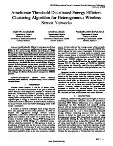
5. Experimental Setup All the existing algorithms LEACH, GCA, and EAERP and proposed algorithm GAECH are implemented in MATLAB. All the algorithms are tested in 20 different network topologies to ensure proper results. Since the location of BS is having a considerable effect on energy consumption, the algorithms are tested in three different scenarios. The three different scenarios vary by the location of BS. In Scenario 1, BS is located at the middle of the network, in Scenario 2 BS at one corner of the network, and in Scenario 3 BS outside of the network. Figures 1, 2, and 3 show the three scenarios, respectively.

Journal of Sensors

5 Table 1: Simulation parameters and values.

100 90

Parameters 𝑛 𝐸elec 𝜀fs 𝜀mp 𝑑0 – distance Initial energy per node Data packet size/control packet size

80 70 60 50 40 30

Values 4000 bits 50 nJ bit−1 10 pJ bit−1 0.0013 pJ bit−1 87 m 1J 500 bytes/25 bytes

10 0

0

10

20

30

40

50

60

70

80

90

100

Figure 2: Scenario 2. 160 140 120 100 80

Average energy consumption per communication round

20 0.06 0.05 0.04 0.03 0.02 0.01 0

5 6 7 8 9 10 11 12 13 14 15 16 17 18 19 20 Number of clusters

Figure 4: Average energy consumption per communication round.

60 40 20 0

0

10

20

30

40

50

60

70

80

90

100

Figure 3: Scenario 3.

The blue spots in Figures 1, 2, and 3 represent the sensor nodes and red spot represents the BS. The transmission energy and reception energy equations are the same as in [15] Transmission Energy 𝐸Tx {𝑛 ∗ 𝐸elec + 𝜀fs ∗ 𝑑 ={ 𝑛 ∗ 𝐸elec + 𝜀mp ∗ 𝑑4 { 2

if 𝑑 < 𝑑0 if 𝑑 > 𝑑0

(12)

Reception Energy 𝐸Rx = 𝑛 ∗ 𝐸elec . 𝐸Tx and 𝐸Rx denote the transmission and reception energy. “𝑛” denotes number of bits to be transmitted; “𝐸elec ” is the electronic energy for node activity. “𝜀fs ” denotes energy dissipation in free space and “𝜀mp ” is the energy dissipation during multipath propagation. “𝑑” represents the distance between two nodes and “𝑑0 ” is the threshold distance to determine the transmission model whether free space or multipath propagation is to be followed. The above parameter values are mentioned in Table 1. From the experimental analysis over 10 different network topologies, it is found that the percentage of CH ranging between 5 and 10 gives optimal energy conservation in the network. When the percentage of CHs is less than 5, it

leads to too much energy consumption for the CH due to more number of cluster members. In another case, when the number of CHs is higher than 10, the cluster formation activities such as CH election broadcasting, requested for member and approval from CH itself, are leading to higher energy consumption among the nodes. In Figure 4, the overall energy consumption in joules in the network is shown for varying number of CHs. In GAECH, the initial random population is generated with 5 to 10 CHs. The cluster head nodes are represented by bit “1” and member nodes are represented by bit “0” and dead sensor nodes are represented by bit “−1.” The selection technique used for GCA, EAERP, and GAECH is elitism. The crossover rate is 𝑝𝑐 = 0.6 and mutation rate 𝑝𝑚 = 0.03. The initial random population is chosen as 20 chromosomes and all the genetic algorithms run for 20 generations. Since the number of generations is fixed, the convergence rate of GAECH is same for all runs. The weight “𝑊” used in GCA is set to 0.5 and the weight values of GAECH are “𝑊1 ” = 0.5, “𝑊2 ” = 0.30, “𝑊3 ” = 0.1, and “𝑊4 ” = 0.1. These weight values have been chosen since they give better results than other combinations. The higher value of “𝑊1 ” may reduce overall energy reduction in the network but leads to First Node Die (FND) soon. Each coefficient value represents the importance level of its component in the fitness function.

6. Simulation Results In the various network configurations, 100 sensor nodes are randomly deployed in the 100 × 100 meter field area. In these configurations, three different scenarios based on

6

Journal of Sensors

Percentage of dead nodes 10 20 30 40 50 60 70 80 90 100

Number of communication rounds LEACH

GCA

EAERP

GAECH

1989 2031 2055 2075 2091 2102 2112 2126 2136 2144

2036 2064 2090 2106 2117 2127 2137 2147 2157 2165

2155 2187 2201 2224 2247 2265 2278 2288 2298 2309

2304 2331 2348 2363 2375 2387 2401 2411 2421 2430

Table 3: Percentage of dead nodes and number of communication rounds in Scenario 2. Percentage of dead nodes 10 20 30 40 50 60 70 80 90 100

Number of communication rounds LEACH

GCA

EAERP

GAECH

2044 2076 2103 2124 2134 2144 2158 2168 2178 2183

2027 2072 2088 2109 2124 2134 2147 2157 2167 2177

2125 2149 2179 2189 2203 2213 2223 2233 2243 2252

2266 2298 2315 2336 2350 2364 2374 2386 2396 2402

Table 4: Percentage of dead nodes and number of communication rounds in Scenario 3. Percentage of dead nodes 10 20 30 40 50 60 70 80 90 100

Number of communication rounds LEACH

GCA

EAERP

GAECH

1877 1911 1944 1957 1972 1992 2003 2022 2032 2038

1913 1946 1973 1995 2018 2033 2043 2055 2069 2081

2035 2055 2079 2110 2129 2142 2153 2163 2173 2184

2206 2234 2250 2271 2285 2301 2312 2332 2345 2354

the location of the BS are verified and the corresponding results are discussed in detail. All the four algorithms are tested and their lifetime is evaluated. The percentage of dead nodes along with the corresponding communication rounds are displayed in Tables 2, 3, and 4.

×102

Number of communication rounds

Table 2: Percentage of dead nodes and number of communication rounds in Scenario 1.

25 24 23 22 21 20 19

0

10

20

LEACH GCA

30 40 50 60 70 80 Number of dead sensor nodes

90

100

EAERP GAECH

Figure 5: Network lifetime for Scenario 1.

6.1. Scenario 1. In this scenario, the BS is located at the middle of the network, that is, (50, 50) 𝑋 and 𝑌 coordinates. Considering FND metrics, GAECH shows improvement in network lifetime by 6.92% better than EAERP, 14.64% better than GCA, and 14.70% better than LEACH. In terms of HND, GAECH is 5.75% higher than EAERP, 12.5% higher than GCA, and 13.4% higher than LEACH. GAECH performs 5% better than EAERP, 12% better than GCA, and 13% better than LEACH in terms of LND. Figure 5 shows the distribution of the number of dead nodes against communication rounds. Table 2 shows the number of communication rounds during every 10% of dead nodes in detailed insight. 6.2. Scenario 2. Since the BS is located at the corner of the network, for some CH the communication distance reduces but for other distant CHs it may increase. By FND metrics, GAECH is 9.52% better than EAERP, 13.44% better than GCA, and 12.18% better than LEACH in increasing network lifetime. When HND is used, GAECH is 6.67% better than EAERP, 10.64% better than GCA, and 10.12% better than LEACH. GAECH shows 6.8% higher performance than EAERP, 10.56% higher performance than GCA, and 10% higher performance than LEACH in terms of LND. Figure 6 shows the distribution of the number of dead nodes against communication rounds. Table 3 shows the number of communication rounds during every 10% of dead nodes in detailed insight. 6.3. Scenario 3. Compared with other two scenarios, since the BS is located outside the network, the number of communication rounds will be relatively low. In terms of FND, GAECH shows a 12.03% improvement in network lifetime compared to EAERP, 20.70% compared to GCA, and 21.11% compared to LEACH. In terms of HND, GAECH is 7.32% better than EAERP, 13.27% better than GCA, and 15.87% better than LEACH. GAECH performs 7.78% higher than EAERP, 13.11% higher than GCA, and 15.50% higher than LEACH in LND metrics. Figure 7 shows the distribution of the number of dead nodes against communication rounds. Table 4 shows the number of communication rounds during every 10% of dead nodes in detailed insight.

Journal of Sensors

7 Average energy consumption per round

25 24 23 22 21 20 19

0

10

20

LEACH GCA

30 40 50 60 70 80 Number of dead sensor nodes

90

100

Number of communication rounds

10

20

LEACH GCA

30 40 50 60 70 80 Number of dead sensor nodes

90

100

EAERP GAECH

0.03 0.02 0.01 0

LEACH

GCA EAERP Clustering algorithms

GAECH

×10−3 5

4 3 2 1 0

Scenario 1

LEACH GCA

Scenario 2 Different scenarios

Scenario 3

EAERP GAECH

Figure 10: Average energy consumption at CH nodes.

×102

Number of communication rounds

0.04

Figure 9: Average energy consumption per communication round.

Figure 7: Network lifetime for Scenario 3.

25 20

0.05

Scenario 1 Scenario 2 Scenario 3

Figure 6: Network lifetime for Scenario 2. ×102 24 23 22 21 20 19 18 17 0

0.06

EAERP GAECH

Average energy consumption at cluster head

Number of communication rounds

×102

1939 1979 1753

1940 1957 1759

2080 2027 1895

2224 22202123

15 10 5 0 LEACH

GCA EAERP Clustering algorithms

GAECH

Scenario 1 Scenario 2 Scenario 3

Figure 8: Stability period (FND) of clustering algorithms.

Figure 8 depicts the stability period, that is, FND occurrence in LEACH, GCA, EAERP, and GAECH algorithms in all the three scenarios, respectively. Since the stability period is an important metric in deciding the reliability of the network, it is shown separately in Figure 8. In the best case, GAECH has achieved 285 higher numbers of communication rounds than LEACH in Scenario 1, 263 rounds than GCA in Scenario 2, and 370 rounds than LEACH in Scenario 3. Figure 9 displays the average energy of the network for a single communication round. LEACH is found to be

consuming more energy than others due to the random and the probable way of election of CH compared to other algorithms. The other genetic based clustering algorithms GCA and EAERP show reduced energy consumption compared to LEACH but the unequal energy consumption between clusters is still affecting their performance. GAECH achieves reduced energy consumption compared to other two genetic algorithms by proper balancing of energy load in each cluster. Figure 10 shows the average energy consumption of a CH node. Due to uneven load between clusters, LEACH, GCA and EAERP have higher energy consumption at their CHs. GAECH properly balances the energy consumption among its CHs through its novel fitness function and comparatively it has less average energy consumption in its CH than other compared algorithms.

7. Conclusion and Future Work The increase in the lifetime of the WSN is achieved in a balanced sense using the proposed algorithm GAECH. The experimental results have shown that GAECH performs better than its other counterparts like GCA, EAERP, and LEACH in three different network scenarios. The increase in performance is distinct when the BS is located far away

8 from the network, which is practically possible in most of the real time applications. As the best case, GAECH shows 21.11% increased lifetime than its counterpart when the BS is located outside of the network. Also GAECH is found to be conserving energy by balancing energy consumption among the clusters. Depending upon the application need, the various weight coefficients mentioned in the fitness function of GAECH can be changed to obtain better results. The future research direction would be around using other parameters like node degree and residual energy of a node in the fitness function.

Conflict of Interests The authors declare that there is no conflict of interests regarding the publication of this paper.

Acknowledgment The authors thank SASTRA University management for its constant motivation towards research.

References [1] A. Hac, Wireless Sensor Networks Designs, John Wiley & Sons, 2004. [2] F. Zhao, J. Liu, J. Liu, L. Guibas, and J. Reich, “Collaborative signal and information processing: an information-directed approach,” Proceedings of the IEEE, vol. 91, no. 8, pp. 1199–1209, 2003. [3] I. F. Akyildiz, W. Su, Y. Sankarasubramaniam, and E. Cayirci, “Wireless sensor networks: a survey,” Computer Networks, vol. 38, no. 4, pp. 393–422, 2002. [4] K. Akkaya and M. Younis, “A survey on routing protocols for wireless sensor networks,” Ad Hoc Networks, vol. 3, no. 3, pp. 325–349, 2005. [5] A. A. Abbasi and M. F. Younis, “A survey on clustering algorithms for wireless sensor networks,” Computer Communications, vol. 30, no. 14-15, pp. 2826–2841, 2007. [6] Y.-H. Zhu, W.-D. Wu, J. Pan, and Y.-P. Tang, “An energy-efficient data gathering algorithm to prolong lifetime of wireless sensor networks,” Computer Communications, vol. 33, no. 5, pp. 639– 647, 2010. [7] M. Ye, C. F. Li, G. H. Chen, and J. Wu, “EECS: an energy efficient clustering scheme in wireless sensor networks,” in Proceedings of the 24th IEEE International Performance, Computing, and Communications Conference (IPCCC ’05), pp. 535–540, April 2005. [8] F. Bajaber and I. Awan, “Adaptive decentralized re-clustering protocol for wireless sensor networks,” Journal of Computer and System Sciences, vol. 77, no. 2, pp. 282–292, 2011. [9] F. Bajaber and I. Awan, “Energy efficient clustering protocol to enhance lifetime of wireless sensor network,” Journal of Ambient Intelligence and Humanized Computing, vol. 1, no. 4, pp. 239– 248, 2010. [10] N. Dimokas, D. Katsaros, and Y. Manolopoulos, “Energy-efficient distributed clustering in wireless sensor networks,” Journal of Parallel and Distributed Computing, vol. 70, no. 4, pp. 371–383, 2010.

Journal of Sensors [11] D. Zhao, K. Long, D. Wang, Y. Yichuan Zheng, and J. Tu, “Energy-saving strategy based on an immunization algorithm for network traffic,” KSII Transactions on Internet and Information Systems, vol. 9, no. 4, pp. 1392–1403, 2015. [12] R. V. Kulkarni, A. F¨orster, and G. K. Venayagamoorthy, “Computational intelligence in wireless sensor networks: a survey,” IEEE Communications Surveys & Tutorials, vol. 13, no. 1, pp. 68– 96, 2011. [13] S. Hussain, A. W. Matin, and O. Islam, “Genetic algorithm for hierarchical wireless sensor networks,” Journal of Networks, vol. 2, no. 5, pp. 87–97, 2007. [14] S. Hussain, O. Islam, and A. W. Matin, “Genetic algorithm for energy efficient clusters in wireless sensor networks,” in Proceedings of the 4th International Conference on Information Technology: New Generations (ITNG ’07), pp. 147–154, IEEE Computer Society, April 2007. [15] W. B. Heinzelman, A. P. Chandrakasan, and H. Balakrishnan, “An application-specific protocol architecture for wireless microsensor networks,” IEEE Transactions on Wireless Communications, vol. 1, no. 4, pp. 660–670, 2002. [16] O. Younis and S. Fahmy, “HEED: a hybrid, energy-efficient, distributed clustering approach for ad hoc sensor networks,” IEEE Transactions on Mobile Computing, vol. 3, no. 4, pp. 366– 379, 2004. [17] S. R. Mudundi and H. H. Ali, “A new robust genetic algorithm for dynamic cluster formation in wireless sensor networks,” in Proceedings of the 7th IASTED International Conferences on Wireless and Optical Communications (WOC ’07), pp. 360–367, Montreal, Canada, June 2007. [18] E. A. Khalil and B. A. Attea, “Energy-aware evolutionary routing protocol for dynamic clustering of wireless sensor networks,” Swarm and Evolutionary Computation, vol. 1, no. 4, pp. 195–203, 2011. [19] D. E. Goldberg, Genetic Algorithms in Search Optimization and Machine Learning, Addison-Wesley, 1989. [20] A. E. Eiben and J. E. Smith, Introduction to Evolutionary Computing, Natural Computing Series, Springer, Berlin, Germany, 2003.

International Journal of

Rotating Machinery

Engineering Journal of

Hindawi Publishing Corporation http://www.hindawi.com

Volume 2014

The Scientific World Journal Hindawi Publishing Corporation http://www.hindawi.com

Volume 2014

International Journal of

Distributed Sensor Networks

Journal of

Sensors Hindawi Publishing Corporation http://www.hindawi.com

Volume 2014

Hindawi Publishing Corporation http://www.hindawi.com

Volume 2014

Hindawi Publishing Corporation http://www.hindawi.com

Volume 2014

Journal of

Control Science and Engineering

Advances in

Civil Engineering Hindawi Publishing Corporation http://www.hindawi.com

Hindawi Publishing Corporation http://www.hindawi.com

Volume 2014

Volume 2014

Submit your manuscripts at http://www.hindawi.com Journal of

Journal of

Electrical and Computer Engineering

Robotics Hindawi Publishing Corporation http://www.hindawi.com

Hindawi Publishing Corporation http://www.hindawi.com

Volume 2014

Volume 2014

VLSI Design Advances in OptoElectronics

International Journal of

Navigation and Observation Hindawi Publishing Corporation http://www.hindawi.com

Volume 2014

Hindawi Publishing Corporation http://www.hindawi.com

Hindawi Publishing Corporation http://www.hindawi.com

Chemical Engineering Hindawi Publishing Corporation http://www.hindawi.com

Volume 2014

Volume 2014

Active and Passive Electronic Components

Antennas and Propagation Hindawi Publishing Corporation http://www.hindawi.com

Aerospace Engineering

Hindawi Publishing Corporation http://www.hindawi.com

Volume 2014

Hindawi Publishing Corporation http://www.hindawi.com

Volume 2014

Volume 2014

International Journal of

International Journal of

International Journal of

Modelling & Simulation in Engineering

Volume 2014

Hindawi Publishing Corporation http://www.hindawi.com

Volume 2014

Shock and Vibration Hindawi Publishing Corporation http://www.hindawi.com

Volume 2014

Advances in

Acoustics and Vibration Hindawi Publishing Corporation http://www.hindawi.com

Volume 2014