International Journal for Uncertainty Quantification, 4 (2): 171–184 (2014)
INFERENCE AND UNCERTAINTY PROPAGATION OF ATOMISTICALLY INFORMED CONTINUUM CONSTITUTIVE LAWS, PART 2: GENERALIZED CONTINUUM MODELS BASED ON GAUSSIAN PROCESSES Maher Salloum1,∗ & Jeremy Templeton2 1
Sandia National Laboratories, 7011 East Avenue, MS 9158, Livermore, California 94550, USA
2
Sandia National Laboratories, 7011 East Avenue, MS 9409, Livermore, California 94550, USA
Original Manuscript Submitted: 07/04/2013; Final Draft Received: 01/27/2014 Constitutive models in nanoscience and engineering often poorly represent the physics due to significant deviations in model form from their macroscale counterparts. In Part 1 of this study, this problem was explored by considering a continuum scale heat conduction constitutive law inferred directly from molecular dynamics (MD) simulations. In contrast, this work uses Bayesian inference based on the MD data to construct a Gaussian process emulator of the heat flux as a function of temperature and temperature gradient. No assumption of Fourier-like behavior is made, requiring alternative approaches to assess the well-posedness and accuracy of the emulator. Validation is provided by comparing continuum scale predictions using the emulator model against a larger all-MD simulation representing the true solution. The results show that a Gaussian process emulator of the heat conduction constitutive law produces an empirically unbiased prediction of the continuum scale temperature field for a variety of time scales, which was not observed when Fourier’s law is assumed to hold. Finally, uncertainty is propagated in the continuum model and quantified in the temperature field so the impact of errors in the model on continuum quantities can be determined.
KEY WORDS: constitutive model, Bayesian inference, Gaussian process, uncertainty, sampling data, continuum model 1. INTRODUCTION In many problems involving nanoscale phenomena, the mathematical models used to form continuum models may not be consistent with the discrete atomistic reality. This inconsistency is related to the closure problem in classical physics in which constitutive relationships are needed to provide unknown fluxes in order to make the equations well-posed. Even when developing computational multiscale models of nano-phenomena, much attention is given to the coupling conditions necessary to exchange information between the mathematical models (e.g., [1]) while relatively little is provided to ensure consistency between the equations. Discrepancy between the two model forms is particularly apparent for problems in which fluctuations are present in the small-scale motions but not representable in the large-scale equations [2]. This difficulty is not insurmountable; Feng and Jones [3] used continuum beam theories modified with energy equipartition from statistical mechanics to develop a continuum model of the vibrations of a carbon nanotube. At larger scales, analytical homogenization (e.g., [4]) is attractive in deriving large-scale equations, including constitutive models, arising from small-scale systems. However, homogenization theory is typically limited to applications with strict scale separation, i.e., it is possible to take the limit of the small-scale parameters to zero while the large scale is invariant. This assumption is violated at the nanoscale (as well as in many macroscale problems,
∗
Correspond to Maher Salloum, E-mail:
[email protected]
c 2014 by Begell House, Inc. 2152–5080/14/$35.00 °
171
172
Salloum & Templeton
e.g., turbulent fluid flows [5] and crystal plasticity [6]). At these scales, difficulties also arise because there are still fluctuations in the quantities of interest. For example, macroscale Navier-Stokes descriptions must give way to fluctuating hydrodynamic models such as the Landau-Lifschitz Navier-Stokes (LLNS) equations [7]. These equations include stochastic forcing terms which make the continuum model consistent with the fluctuations present due to atomic motions [8]. It has been shown by Donev et al. [9] that using the LLNS equations is necessary to perform coupled continuum/Direct Simulation Monte Carlo (DSMC) particle simulations as opposed to using the traditional Navier-Stokes equations. While not focused on developing continuum models, several efforts have attempted to extract the continuum equivalents of mechanical properties from atomistic simulations. Irving and Kirkwood [10] proposed the original such procedure, which has since been greatly expanded. These approaches often produce results which diverge from classical macroscale continuum models, e.g., elasticity, for nanoscale phenomena. Unsurprisingly, attempts to use established constitutive model forms for nanostructures have met with much difficulty and are the subject of active research, for example models of carbon nanotubes [11]. The proposed approach in this work builds on our previous effort [12] in which constitutive laws for large scale equations are statistically inferred from smaller scale realizations. In Part 1 of this series [12], Bayesian inference was used to estimate the coefficients of a polynomial chaos expansion (PCE) model of the thermal conductivity κ. An assumed form was used based on Fourier’s law: q = κ =
−κ∇T A − BT
(1)
In the above equation, q is the heat flux, T the temperature, and the parameters A and B are each represented by a PCE informed by small-scale molecular dynamics (MD) simulations with prescribed boundary conditions [13]. The most significant issue was that many realizations produced a negative value for κ, violating the solvability constraints of the continuum diffusion equation. (This inconsistency manifests itself in some macroscale physics as well; for example, it is the reason that plane averaging is used in the dynamic Smagorinsky turbulence model [14]). A Rosenblatt transformation provided mitigation and resulted in P(κ > 0) = 1, but was responsible for a biased estimate of the correct solution. Specifically, when the inferred continuum model was compared to an equivalent large MD calculation, the estimate converged from below with increasing sample size. At the microscale, heat is transported in crystal lattices by phonons: lattice wave packets which travel in random directions, but preferentially in the opposite direction of the temperature gradient [15]. Fourier’s law is only expected to hold when this condition is met. For more details, the reader is referred to discussions on the fluctuation-dissipation theory [16]. Therefore, any appropriate thermodynamic average will result in κ > 0 and the resulting heat flux will be the difference between phonons traveling with the temperature gradient and those traveling against it. While these averages may be approached computationally through increasing averaging windows, they can never be completely realized, and hence there will always be an inconsistency between molecular simulations and a continuum description predicated on Fourier’s law. This present paper focuses on a method which, empirically, produces an unbiased estimator for the heat flux. It allows for negative heat fluxes with a frequency consistent with the distribution of phonons in the system and the coarse-graining operators connecting atomistic to continuum models. In the process, Fourier’s law must be jettisoned. Instead, a Gaussian process emulator with a nonparametric error model is used to represent the heat flux q rather than the conductivity κ. The inferred heat flux may then be used in a continuum simulation where negative heat fluxes are possible. The MD simulations are the same as used in Part 1, including the “local” and “global” sampling strategies, so the details are not repeated here. However, Fig. 1 shows that in many cases, a heat flux counter to that expected from Fourier’s law does occur, providing motivation for the approach taken in this work. At high values of the time averaging window tw , we notice that when using a local sampling approach, the data span a limited region in the {T, ∇T } space. The data cover a bigger range in the {T, ∇T } space in a more uniform manner using a global sampling approach. In the next section, we provide the mathematical formulation for the Gaussian Process (GP) [17–19] representation used for the heat flux, followed by the Bayesian inference methodology to infer the heat flux surface. We also discuss
International Journal for Uncertainty Quantification
Generalized Continuum Models based on Gaussian Processes
173
tw =128 ps
tw =32 ps 8
8
8
x 10
x 10
4
4
2
2
2
0 −2 −4 −5
q (W.m−2)
4
q (W.m−2)
0 −2 −4 −5
8 0 x 10 ∇T (K.m−1)
45 55
5
45
8
x 10
50
0 ∇T (K.m−1)
T (K)
9
0 −2 −4 −5
5
55
0 ∇T (K.m−1)
T (K)
9
x 10
0.5
0.5
0.5
q (W.m−2)
1
−1 −2 9 0 x 10 ∇T (K.m−1)
0 −0.5 −1 −2
40 50 60 2
9
x 10
55 T (K)
0 −0.5 −1 −2
40
0
∇T (K.m )
50 2
9
x 10
T (K)
40
0 ∇T (K.m−1)
60
−1
T (K)
5
x 10
1
−0.5
50
9
x 10
1
0
45
8
x 10
50
q (W.m−2)
q (W.m−2)
x 10
q (W.m−2)
tw =512 ps
50 60 2
T (K)
FIG. 1: Plots showing short-time averages of the temperature, temperature gradient, and heat flux. Results are generated: (top row) using a local sampling approach from MD simulations for THOT = 60 K, TCOLD = 40 K (see Part 1 [12]), and (bottom row) from MD simulations with a global sampling approach, for La = 53 nm when the statistical steady state is reached for different time averaging window widths tw , as indicated. the solvability criterion for this formulation of the heat transport equations. An ad hoc method is shown to transform the raw GP into one satisfying this constraint. Section 3 presents the GP results for our example problem and comparisons are made between the uncertain continuum equations and a corresponding MD simulation to demonstrate the unbiased estimate produced by this formulation. The effect of the sampling approach on the inferred heat conduction constitutive law is also studied and reported in this section. Some concluding thoughts are offered in Section 4. 2. MATHEMATICAL MODEL FORMULATION In this section we describe the mathematical formulation for the inferred conductivity with specific implementation details. Major steps of the inference process are illustrated in Fig. 2. 2.1 Emulating the Heat Conduction Constitutive Law by a GP We build the heat conduction constitutive law as a function f (·) that emulates the relationship between heat flux q, temperature T , and temperature gradient ∇T , namely q = f (T, ∇T )
(2)
The data {Ti , ∇Ti } extracted from the MD simulation form the design points based on which the emulator is built. The qi extracted from the MD simulations are the output of the emulator and constitute the training data for the inference
Volume 4, Number 2, 2014
174
Salloum & Templeton
FIG. 2: Schematic illustrating the major steps of the constitutive law inference process. of f (·). The T , ∇T , and q data are collected when the a statistical steady state is reached in the MD simulation of the 1D bar. Moreover, these data are noisy with a level that decreases with the averaging time scale according to the central limit theorem (CLT). In such cases, the Gaussian assumption is reasonable with regard to the statistical discrepancy from the true value of q [18]. Therefore, we represent the emulator f (·) as a single-output GP. We use Bayesian inference to construct this GP since it is suitable to handle noisy data as well as other heterogeneous sources of uncertainty, and because it provides a heat flux estimate uncertainty certificate (unlike maximum likelihood estimate methods) regardless of how noisy and scattered the T , ∇T , and q data are [20–22]. We denote by θTi = {Ti , ∇Ti } ∈ Rp . Hence the design points matrix and training data vector are given by θT qT
= =
{θ1 , . . . , θN } ∈ RN ×p {q1 , . . . , qN } ∈ RN
(3)
where p = 2 and N is the number of short-time averaged data points extracted from the MD simulations. We assume that the uncertainty in the emulator output can be described as a GP. There are different mathematical formulations for a GP in the literature [18]. In this paper, we choose the most general formulation of O’Hagan et al. [17]. Hence the prior knowledge about f (·) is given by a GP of mean E(·) and covariance Σ(·, ·) [17, 23] E(θ) Σ(θ, θ0 )
= h(θ)T · β = σ2 C(θ, θ0 )
(4)
where h(·) ∈ Rv is a function of the input θ, i.e., the temperature and the temperature gradient, β ∈ Rv is a vector of coefficients to be determined, σ2 is a scale factor to be determined, and C(·, ·) is given by £ ¤ C(θ, θ0 ) = exp −(θ − θ0 )T Ψ(θ − θ0 ) + s2 δ(θ, θ0 ) (5) where s2 is a noise term that can be deduced from the observed q data (see Fig. 1), and δ is the Kronecker symbol. The noise amplitude given by s2 depends on the temperature in the MD simulation [12] but we assume that it is constant and equal to the variance of the MD heat flux data. There is no specific rule to choose the function h(·). However, it is should be chosen such that it incorporates any knowledge about the relationship between the output q and the input θ. In this study, we set h(·) as h(θ)T
=
{1, T, ∇T, T ∇T, T 2 , ∇T 2 , T 2 ∇T, T ∇T 2 }
(6)
International Journal for Uncertainty Quantification
Generalized Continuum Models based on Gaussian Processes
175
such that v = 8. The relationship in Eq. (6) can be thought of as a generalization of the Fourier law between the heat flux q, the temperature T , and the temperature gradient ∇T in that the heat flux is a more general function of the temperature and temperature gradient, rather than the less general product of a temperature-dependent conductivity and the temperature gradient normally associated with Fourier’s law. The matrix Ψ ∈ Rp×p is diagonal and contains the data roughness parameters that we determine as described later in this section. Unlike the parametric Bayesian approach [12], the GP formulation allows for model inadequacy errors and accounts for the correlation between the output and the data through the covariance Σ in Eq. (4). Based on a Gaussian assumption, we write
where
P(q|β, σ2 , Ψ) ∼ N (Hβ, σ2 A)
(7)
H = {h(θ1 ), . . . , h(θN )}T ∈ RN ×v
(8)
Ai,j={1,...,N } = C(θi , θj )
(9)
We now would like to update our belief about the output f (·) represented by Eq. (4) with the data q extracted from the MD simulations at the design points θ [see Eq. (3)]. Given the likelihood function in Eq. (7) and the prior knowledge on f (·) given by Eq. (4), we apply Bayes theorem [24] and derive an analytical expression for the conditional posterior distribution of f (·) as f (·)|q, β, σ2 , Ψ ∼ N (m(·), σ2 c(·, ·)) (10) where m(θ) = c(θ, θ0 ) = t(θ)T =
h(θ)T β + t(θ)T A−1 (q − Hβ) C(θ, θ0 ) − t(θ)T A−1 t(θ0 )T {C(θ, θ1 ), . . . , C(θ, θN )}
(11)
We now include any prior knowledge about β and σ2 . We assign an improper uniform prior to the coefficients of β on [−∞, +∞] [21, 24]. For σ2 , leveraging the fact that there is a priori complete ignorance about its value except that it cannot be negative, we assume a Jeffrey’s prior such that P(β, σ2 ) ∼
1 σ2
(12)
After a series of Bayes theorem applications on Eqs. (7) and (12), and after marginalizing over β and σ2 , we obtain a Student-t distribution for the final posterior ˆ 2 V (·, ·)) P(f (·)|q, Ψ) ∼ S(N − v, f¯(·), σ where
f¯(θ) V (θ, θ0 ) ˆ β ˆ2 σ
ˆ + t(θ)T A−1 (q − Hβ) = h(θ)T β = C(θ, θ0 ) − t(θ)T A−1 t(θ0 )T £ ¤¡ ¢−1 £ ¤T + h(θ)T − t(θ)T A−1 H H T A−1 H h(θ0 )T − t(θ0 )T A−1 H ¡ ¢−1 T −1 H A q = H T A−1 H h ¡ ¢−1 T −1 i H A q q T A−1 − A−1 H H T A−1 H = N −v−2
(13)
(14)
Because of the normality of the GP and the priors we chose, we can derive analytical expressions for this Bayesian inference problem. However, in many other cases one cannot and has to resort to more expensive Markov Chain Monte Carlo (MCMC) methods [21]. The analytical framework makes the inference more attractive and easier to implement. The only unknowns that remain in the previous derivation are the roughness parameters (the diagonal elements of the matrix Ψ) since the derivation above is conditional on Ψ that has an intrinsic dependence on the data θ and q. Inferring
Volume 4, Number 2, 2014
176
Salloum & Templeton
roughness parameters often leads to ill-posedness and is not tractable analytically. Hence, we fix these unknowns and choose their values as the ones that maximize the following likelihood function [19, 23] ˆ v−N L(Ψ|θ, q) ∝ |A|−1/2 |H T A−1 H|−1/2 σ
(15)
Further details about this GP emulation can be found in [23]. According to this derivation, we can write Eq. (2) as [17] p ˆ 2 V (θ, θ) ξ (16) q(θ) = f¯(θ) + σ | {z } | {z } q¯
σq
where θ = ξ ∼
{T, ∇T }, S(N − v, 0, 1)
(17)
For N > 30, a Student-t process can be easily approximated by a GP [21], i.e., ξ ∼ N (0, 1). 2.1.1 Enforcing the Well-Posedness of the Constitutive Law In Eq. (16), the heat flux has two components. The first term on the right-hand side is the mean of the flux as a function of temperature and temperature gradient, while the second term encompasses the uncertainty due to the intrinsic fluctuations in the atomistic data. The mathematics of the continuum diffusion equation require a positive thermal conductivity everywhere. However, the atomistic data used to inform the procedure described above produce negative values as, due to nanoscale fluctuations, the heat flux can align with the temperature gradient with nonzero probability [12]. In other words, the function f in Eqs. (2) and (16) is not guaranteed to strictly decrease as a function of the temperature gradient ∇T . In order to guarantee that well-posed solutions exist for the continuum heat transport equations, we propose a smoothing operation on the function f (·) to allow the heat flux to follow the opposite direction of the temperature gradient. According to Eq. (2), we require that ∂q ≤0 ∂∇T
for all T and ∇T
(18)
Due to the difficulty of enforcing this type of constraint on the GP emulator, an alternate ad hoc method is used to enforce the needed behavior of the heat flux to serve as a proof of concept of this method (we defer a more rigorous approach to constraint-realizing GPs to a future effort). The parabolic partial differential equation (PDE) operator is known to have a transient smoothing effect on a given function. We propose to solve the following parabolic PDE: ∂q ∂2q ∂2q = + s ∂τ ∂T 2 ∂∇T 2
in [0, ∇Tmax ] × [Tmin , Tmax ]
(19)
as a function of some fictitious time τ until Eq. (18) is satisfied, setting s = 10 to bias the smoothing toward the ∇T dimension. We first assume that the heat flux q is defined for a range of T ∈ [Tmin , Tmax ] and ∇T ∈ [0, ∇Tmax ]. This range can be set following the range of T and ∇T in the atomistic data. Given this range, suitable boundary conditions are needed to solve Eq. (19). For ∇T = 0, we set q = 0 as required by the continuum constitutive law. For the remaining boundaries Tmin , Tmax , and ∇Tmax , the derived heat flux in Eq. (16) incurs the following relationships: q q
= =
g1 (∇T ) g2 (∇T )
q
=
g3 (T )
for T = Tmin for T = Tmax for ∇T = ∇Tmax
(20)
where g1 , g2 , and g3 are nonmonotonic functions due to the fluctuating nature of the emulator surface q. Thus we perform linear curve fits on these functions and impose them as conditions at their corresponding boundaries. We denote these linear fits by g1s , g2s , and g3s . The full smoothing problem is thus solved using Eq. (19) and the following boundary conditions:
International Journal for Uncertainty Quantification
Generalized Continuum Models based on Gaussian Processes
q = g1s (∇T ) q = g2s (∇T )
177
for T = Tmin for T = Tmax
q = g3s (T ) for ∇T = ∇Tmax q = 0 for ∇T = 0
(21)
The solution of this problem is denoted by qs and referred to as the smoothed heat flux surface. It will be used to solve a continuum scale heat conduction problem as described in Section 3. 2.2 The Inferred Heat Flux Surface The mean of the inferred continuum scale mean heat flux, q¯(T, ∇T ) [see Eq. (16)] can be represented by a surface, shown in Figs. 3 and 4 (top row). Using a “local” sampling strategy, this surface exhibits significant fluctuations that decrease with the time averaging window tw because the fluctuations in the MD training data decrease with tw , as
FIG. 3: Plots showing (top row) the mean surface f¯(·) [see Eq. (14)] of the GP (middle row) the smoothed mean surface, and (bottom row) the variance of the GP. Results are generated using a local sampling approach from MD simulations for THOT = 60 K, TCOLD = 40 K, and La = 53 nm (see Part 1 [12]) with N = 64 short-time averaged values of the flux, temperature, and temperature gradient and for different time averaging window widths tw , as indicated. Note the scale of the variance is decreasing with increasing tw .
Volume 4, Number 2, 2014
178
Salloum & Templeton
FIG. 4: Plots showing (top row) the mean surface f¯(·) [see Eq. (14)] of the GP (middle row) the smoothed mean surface, and (bottom row) the variance of the GP. Results are generated from MD simulations with a global sampling approach for La = 53 nm (see Part 1 [12]), N = 64 short-time averaged values of the flux, temperature, and temperature gradient and for different time averaging window widths tw , as indicated. The dashed line in the top left panel delineates the {T, ∇T } range covered by the local sampling approach. Note the scale of the variance is decreasing with increasing tw . depicted in Fig. 1. The {T, ∇T } range covered in a local sampling approach is significantly smaller than the one covered in the global sampling approach as visualized by the dashed line in Fig. 4 (top left). Hence, fluctuations are less likely to happen using a global sampling approach since the training data spread over a bigger {T, ∇T } range granting the emulator a smoother interpolation. After enforcing the well-posedness of the constitutive law, the oscillations in the heat flux surface are eliminated for all values of tw as shown in the q¯s plots in Figs. 3 and 4 (middle row). The effect of this smoothing is nearly absent when the global sampling approach is used since deviations from the solvability constraints are much smaller in the raw heat flux surface q¯. Enforcing the well-posedness under a global sampling approach is only present for high temperatures and temperature gradients as shown in Fig. 4. This is due to the linear fit for the boundary condition used in the smoothing process, as described in Section 2.1.1, and could be improved with a more accurate treatment at the boundaries.
International Journal for Uncertainty Quantification
Generalized Continuum Models based on Gaussian Processes
179
The uncertainty σq in the inferred heat flux is plotted in Figs. 3 and 4 (bottom row). This uncertainty is due to the inadequacy of the relationship in Eq. (6) as well as the noise present in the MD data and represented by s2 [see Eq. (5)]. There is a substantial decrease in this uncertainty for increasing tw throughout the whole {T, ∇T } space and for both sampling approaches, due to the significant reduction in the MD data noise with more averaging. When using a local sampling approach, the uncertainty drops in a restricted area in the {T, ∇T } space where the training data are located. The uncertainty is more uniform in the {T, ∇T } space using a global sampling approach since the training data are more uniformly spread as depicted in Fig. 1. 3. RESULTS 3.1 Simulating the Continuum Using the Uncertain Constitutive Law In this section we propagate the constitutive law derived in the previous section into a 1D continuum problem. Figure 5 shows the schematic of such a continuum simulation. The length scale of this simulation should be at least an order of magnitude bigger than the atomistic simulation length scale, i.e., Lc ≥ 10La , to get into a regime where the continuum formulation is valid. We discretize the continuum simulation domain such that the local shape functions spread over a length scale comparable to the atomistic simulation domain size, resulting in the mesh size h satisfying 2h = La . Consistent with the MD simulation, we impose Dirichlet boundary conditions on the continuum domain. Given the heat flux constitutive law in Eq. (16), the PDE governing thermal transport for the continuum scale 1D bar is written as ∂qs (T, ∇T ) ∂T = (22) ρcp ∂t ∂x At each time step, the temperature gradient is computed from the current temperature field. The heat flux is then interpolated in qs (see Section 2.1.1) at all mesh points enabling the computation of the temperature field at the next time step. 3.2 Continuum Simulation using the Mean Heat Flux Surface To demonstrate the model in an application, we use the inferred constitutive law in a continuum scale simulation of a 1D bar as described in Sections 3.1 and 2.1.1. We select the 1D bar length to be 10 times the one used in the atomistic simulation such that Lc = 10La = 0.53 µm. During the simulation, we assign Dirichlet boundary conditions Tc,1 = 60 K and Tc,N = 40 K that are held fixed throughout the simulation. In order to validate the model, we also simulated the same continuum scale heat transfer in the 1D bar directly using MD as described in Part 1 [12]. We denote this large validation simulation by the “validation MD simulation.” We compare the results of these two simulations of the large 1D bar in Fig. 6 in terms of the mean of the temperature computed based on the mean heat flux surface q¯s , which in turn is inferred according to local and global sampling approaches. Unlike the fully parametric inference of the constitutive law [12], there is good agreement between the means of the temperature computed using the two approaches for all time averaging windows tw considered in this
FIG. 5: Schematic showing the 1D continuum simulation domain. Dirichlet boundary conditions are imposed on the bar, as indicated. The bar has a length Lc = 10La = 0.53 µm. The black dots represent mesh points such that the mesh size is equal to La /2 = 26.5 nm (see Part 1 [12]).
Volume 4, Number 2, 2014
180
Salloum & Templeton
“global” sampling
50
50
48
48
46
46
T (K)
T (K)
“local” sampling
44
Continuum tw = 32 ps (fully parametric inference of Part 1)
42 40 0
0.1
0.2
44 Validation MD Continuum tw = 32 ps Continuum tw = 128 ps Continuum tw = 512 ps
42 40 0
0.3
0.1
60
Validation MD Continuum tw = 32 ps Continuum tw = 128 ps Continuum tw = 512 ps
55
T (K)
T (K)
0.3
60
55
50
45
40 0
0.2
Time (µs)
Time (µs)
50
45
0.2
0.4
0.6
40 0
0.2
x (µm)
0.4
0.6
x (µm)
FIG. 6: Plots showing (top row) the temporal evolution of the temperature in the middle of a continuum scale 1D bar (x = 0.26 µm), and (bottom row) the temperature field in the bar at steady state. Results are generated using two approaches: (blue, green, and red lines) by propagating the smoothed mean heat flux surface q¯s inferred from MD simulations into a continuum simulation, and (black circles) the validation MD simulation of the continuum scale bar (Lc = 0.53 µm). The error bars represent the calculated standard deviation in the temperature. Results are obtained with an initial conditions Tinit = 40 K and for continuum boundary conditions Tc,1 = 60 K and Tc,N = 40 K (see Part 1 [12]). The heat flux surface is extracted using a local sampling approach from MD simulations for THOT = 60 K and TCOLD = 40 K (left column), and a global sampling approach (right column) and for N = 64 and different time averaging windows tw , as indicated. The dashed line denotes the result generated with a heat conduction law obtained using a fully parametric inference from Part 1. study. Using GP emulation of the heat flux as a function of temperature and temperature gradient has empirically greatly reduced the bias in the predicted temperature at the continuum scale. 3.3 Uncertainty Quantification in the Continuum Simulation Finally we propagate the full expression of the inferred heat flux surface into the continuum simulation. In this exercise, random samples are drawn from Eq. (16) assuming that ξ ∼ N (0, 1). We enforce the well-posedness of each sample of the heat flux surface such that it can be used as constitutive law to solve for the temperature field in the
International Journal for Uncertainty Quantification
Generalized Continuum Models based on Gaussian Processes
181
continuum scale 1D bar. Results for each sample are obtained with initial conditions Tinit = Tc,N = 40 K and for continuum boundary conditions Tc,1 = 60 K and Tc,N = 40 K that are held constant throughout the simulation. The probability density function (PDF) of the temperature can therefore be built at each time step and over all the finite element mesh points. Figure 6 shows the standard deviation of the temperature in terms of error bars for different time averaging windows. The standard deviation decreases with tw , as expected. For different times, we report the PDF of the temperature in the middle of the bar in Fig. 7. Initially, the uncertainty in the temperature increases as represented by the spread in the PDF. As the system approaches the steady state, the trend is reversed and the PDF converges to a steady state distribution around t = 0.48 µs. At steady state, the global sampling approach results in a narrower PDF indicating a more accurate temperature prediction since it covers a bigger range of temperature and temperature gradient and results in smoother interpolations. 4 t=0.0075 µs t=0.015 µs t=0.03 µs t=0.06 µs t=0.12 µs t=0.24 µs t=0.48 µs t=0.96 µs
3.5
PDF(T )
3 2.5 2 1.5 1 0.5 0
40
41
42
43
44
45
46
47
48
49
45
46
47
48
49
T (K) 4 t=0.0075 µs t=0.015 µs t=0.03 µs t=0.06 µs t=0.12 µs t=0.24 µs t=0.48 µs t=0.96 µs
3.5 3
PDF(T )
2.5 2 1.5 1 0.5 0
40
41
42
43
44 T (K)
FIG. 7: Plots showing the temporal evolution of the PDF of the temperature in the middle of a continuum scale 1D bar (x = 0.26 µm). Results are generated by propagating 5000 samples of smoothed heat flux surface qs inferred from MD simulations into a continuum simulation of a 1D bar (Lc = 0.53 µm). Results are obtained for Tc,1 = 60 K and Tc,N = 40 K (see Part 1 [12]). The heat flux surface is extracted using a local sampling approach from MD simulations for THOT = 60 K and TCOLD = 40 K (top) and a global sampling approach (bottom) for tw = 128 ps and N = 64.
Volume 4, Number 2, 2014
182
Salloum & Templeton
3.4 Discussion Similarly to Part 1 of this study [12], the Bayesian inference of a GP emulator of the heat flux as a function of temperature and temperature gradient from MD simulations data resulted in a heat conduction constitutive law. Inference using either a local or a global sampling approach resulted in an accurate prediction of the spatial and temporal mean temperature field in a one-dimensional continuum scale heat transfer problem. The generation of the MD data in the global sampling approach considered in this study costs 25 times more than the local sampling approach since more MD simulations had to be performed [12]. This additional cost incurred different benefits to the inference of the constitutive law. First, the heat flux surface inferred using a global sampling approach occupies a bigger area in the {T, ∇T } space, allowing us to solve heat transfer problems with a variety of temperature ranges. Secondly, the data obtained in a global sampling approach are more uniformly distributed in the {T, ∇T } space. This feature is crucial to minimize the model error when inferred as a GP. Third, the effort to enforce the well-posedness of the constitutive law is minimal in a global sampling approach since the model error is decreased and the fluctuations in the heat transfer surface are significantly decreased. The choice between a local and a global sampling depends on the scope of the continuum scale problem to be addressed, e.g., the temperature ranges and acceptable levels of uncertainty. There is a trade-off between spending an additional computational cost to generate data in a global sampling setting and affording restricted ranges of temperature with increased levels of uncertainty.
4. CONCLUSION This paper presents a proof-of-concept study for a mathematical formulation in which generalized constitutive models are inferred for use with continuum models of nanoscale phenomena. In this paradigm, a continuum model is connected to an atomistic model through inference of appropriate constitutive relationships. In Parts 1 and 2 of this study we have identified the trade-offs amongst different methodologies to realize this type of nanoscale continuum model. First and foremost, there is a significant advantage in predictive ability to inferring a nonparametric model of constitutive law as opposed to fitting an assumed form. In general, there is no guarantee that prescribed constitutive relationships are consistent with the behavior of the atomic data from which they are generated. Even small inconsistencies can lead to numerical instabilities when the solvability criteria of the continuum equation are violated; in the case of the heat equation, even one realization in which the heat flux is counter to the temperature gradient can cause the continuum solution to be unachievable. While the more flexible constitutive relationships are advantageous, they are not without additional cost. It is important to understand the new solvability criteria associated with the generalized PDE and incorporate these criteria into the GP representation of the constitutive information. In the heat transfer example, the solvability criterion is already known, but the complex equations with additional terms in the parameter space the existence and uniqueness conditions may require new theoretical developments. Additionally, incorporation of constraints into the GP representation is nontrivial. In order to evaluate the soundness of the overall method, we resorted to an ad hoc method to smooth the emulator function and to satisfy the constraints on the heat flux. More rigorous techniques for constraint enforcement will be the focus of future work. Further, improved means to differentiate the uncertainty due to limited data from the physical uncertainty in the GP will enable more meaningful uncertainty quantification within this paradigm as well as improve its predictive ability. Finally, we have considered two sampling strategies to understand how changes to the underlying small-scale data lead to differences in large-scale behavior. It has been determined that more localized samples are less accurate but also less expensive than a global evaluation of the parameter space. In this case, the global study was an order of magnitude more expensive than the more targeted sampling strategies, but had much better performance than when the smaller cases required extrapolation to provide data to the continuum. While unsurprising, this result points to the need to either intelligently choose the initial samples to correspond exactly to the parameter space which will be encountered by the larger scales, or to provide a means for adapting an initial sample. It should be noted that the entirety of the small MD samples was obtained at 1/25th the cost of the validation MD simulation, demonstrating the potential of this method to not only improve accuracy, but performance as well.
International Journal for Uncertainty Quantification
Generalized Continuum Models based on Gaussian Processes
183
ACKNOWLEDGMENTS Sandia National Laboratories is a multiprogram laboratory managed and operated by Sandia Corporation, a wholly owned subsidiary of Lockheed Martin Corporation, for the US Department of Energy’s National Nuclear Security Administration under contract DE-AC04-94AL85000. This work was partially supported by the Laboratory Directed Research and Development (LDRD), and its support is gratefully acknowledged. The authors would like to thank Jon Zimmerman for helpful discussions regarding the extraction of continuum properties from MD. The authors also thank Dr. Khachik Sargsyan and Dr. Laura Swiler for their constructive feedback on a draft of this paper.
REFERENCES 1. Miller, R. and Tadmor, E., A unified framework and performance benchmark of fourteen multiscale atomistic/continuum coupling methods, Model. Simul. Mater. Sci. Eng., 17:053001, 2009. 2. Wagner, G., Jones, R., Templeton, J., and Parks, M., An atomistic-to-continuum coupling method for heat transfer in solids, Comput. Methods Appl. Mech. Eng., 197:3351–3365, 2008. 3. Feng, E. and Jones, R., Equilibrium thermal vibrations of carbon nanotubes, Phys. Rev. B, 81(12):125436, 2010. 4. Bensoussan, A., Lions, J., and Papanicolaou, G., Boundary layers and homogenization of transport processes, Pub. Res. Inst. Math. Sci., 15(1):54–156, 1979. 5. V¨olker, S., Moser, R., and Venugopal, P., Optimal large eddy simulation of turbulent channel flow based on direct numerical simulation data, Phys. Fluids, 14(10):3675–3691, 2002. 6. Horstemeyer, M., Integrated Computational Materials Engineering for Metals, Wiley & Sons, Inc., New York, 2012. 7. Landau, L. and Lifshitz, E., Fluid Mechanics, Elsevier, Amsterdam, 1959. 8. Mashiyama, K. and Mori, H., Origin of Landau-Lifshitz hydrodynamic fluctuations in non-equilibrium systems and a new method for reducing Boltzmann-equation, J. Stat. Phys., 18(4):385–407, 1978. 9. Donev, A., Bell, J. B., Garcia, A. L., and Alder, B. J., A hybrid particle-continuum method for hydrodynamics of complex fluids, SIAM Multiscale Model. Simul., 8:871–911, 2010. 10. Irving, J. H. and Kirkwood, J. G., The statistical mechanical theory of transport processes. IV. The equations of hydrodynamics, J. Chem. Phys., 18:817–829, 1950. 11. Qian, D., Wagner, G., Ruoff, R., Yu, M., and Liu, W., Mechanics of carbon nanotubes, App. Mech. Rev., 55(2):495–533, 2002. 12. Salloum, M. and Templeton, J., Inference and uncertainty propagation of atomistically informed continuum constitutive laws, Part 1: Bayesian inference of fixed model forms, Int. J. Uncert. Quantif., 4(2):151–170, 2014. 13. Templeton, J., Jones, R., and Wagner, G., Application of a field-based method to spatially varying thermal transport problems in molecular dynamics, Modeling. Simul. Mater. Sci. Eng., 18:1–22, 2010. 14. Ghosal, S., Lund, T., Moin, P., and Akselvoll, K., A dynamic localization model for large-eddy simulation of turbulent flows, J. Fluid Mech., 286:229–255, 1995. 15. Srinivasta, G., The Physics of Phonons, Taylor & Francis Group, London, 1990. 16. Reif, F., Fundamentals of Statistical and Thermal Physics, Waveland Press, Inc., New York, 1965. 17. Oakley, J. and O’Hagan, A., Bayesian inference for the uncertainty distribution of computer model outputs, Biometrika, 89(4):769–784, 2002. 18. Rasmussen, C. and Williams, C., Gaussian Processes for Machine Learning, MIT Press, Cambridge, MA, 2006. 19. Bastos, L. and O’Hagan, A., Diagnostics for Gaussian process emulators, Technometrics, 51(4):425–438, 2009. 20. Rizzi, F., Salloum, M., Marzouk, Y., Xu, R., Falk, M., Weihs, T., Fritz, G., and Knio, O., Bayesian inference of atomic diffusivity in a binary Ni/Al system based on molecular dynamics, SIAM Mult. Model. Simul., 9:486–512, 2011. 21. Salloum, M., Sargsyan, K., Najm, H., Debusschere, B., Jones, R., and Adalsteinsson, H., A stochastic multiscale coupling scheme to account for sampling noise in atomistic-to-continuum simulations, SIAM. Mult. Model. Simu., 10(2):550–584, 2011.
Volume 4, Number 2, 2014
184
Salloum & Templeton
22. Rizzi, F., Najm, H., Debusschere, B., Sargsyan, K., Salloum, M., Adalsteinsson, H., and Knio, O., Uncertainty quantification in MD simulations. Part I: Forward propagation, SIAM Mult. Model. Simul., 10(4):1428–1459, 2011. 23. Stephenson, G., Using derivative information in the statistical analysis of computer models, PhD Thesis, University of Southampton, 2010. 24. Sivia, D. and Skilling, J., Data Analysis, A Bayesian Tutorial, Oxford Science, 2 ed., Oxford, 2006.
International Journal for Uncertainty Quantification