of Petri nets and a method to generate finite samples from such a class. The classes may contain infinitely many Petri nets, each net with its own probability to be ...
Generating Benchmarks by Random Stepwise Refinement of Petri Nets Kees M. van Hee and Zheng Liu Department of Mathematics and Computer Science Eindhoven University of Technology P.O. Box 513, 5600 MB Eindhoven, The Netherlands {k.m.v.hee, z.liu3}@tue.nl
Abstract. The quality of algorithms is often determined by benchmarking, i.e., testing the algorithm on a predetermined data set. In contrast to traditional benchmarking, with fixed data set, we present a way to generate random sets of test data. In this paper we present random classes of Petri nets and a method to generate finite samples from such a class. The classes may contain infinitely many Petri nets, each net with its own probability to be generated. This generation method is based on stepwise application of construction rules such as refinement rules. Each random class of Petri nets has a probability distribution for each of its characteristics. We illustrate the approach by estimating this distribution for some simple characteristics. Keywords: Petri nets, benchmarking, random graphs
1
Introduction
In computer science research we often lack a method to evaluate the quality of an algorithm in an analytical way. The quality may concern the efficiency of the algorithm (how fast is a solution found) or the effectiveness (how good is the solution found). Although it is sometimes possible to give bounds for the worst case behavior, it is seldom possible to determine the average-case behavior analytically. What we normally do is fixing a set of test data as benchmark and then we test the algorithm on that set, which is called benchmarking. Generally a benchmark is either pre-defined or generated. Both have disadvantages [15]. Pre-defined datasets are designed to be representative examples in a particular domain. Researchers evaluate new algorithms with respect to such a fixed benchmark, but how good are they if applied to other test data? In order to increase the quality of benchmarking we will consider methods to generate random benchmarks, which are samples from an infinite set of tests, each having its own probability of being selected for a sample. Note that it is impossible to have an infinite set of tests each having the same probability, so the probabilities of the tests have to be non-uniform. Due to the fast increasing computing power we are able to generate samples that are so big that all non-selected tests together have a probability below some chosen bound. This allows us to obtain statistical statements of the quality of an algorithm.
Recent Advances in Petri Nets and Concurrency, S. Donatelli, J. Kleijn, R.J. Machado, J.M. Fernandes (eds.), CEUR Workshop Proceedings, ISSN 1613-0073, Jan/2012, pp. 403–417.
404 Petri Nets & Concurrency
van Hee and Liu
In this paper we focus on Petri nets and algorithms to compute their characteristic properties. Hence we define random classes of Petri nets. Such a class contains Petri nets with some structural property, like free choice nets. There may be infinite number of nets in one class. Each net in a class has its own probability of being selected for a benchmark. Petri nets are used to model complex processes [11], for example computational processes in a computer system or business processes within or between enterprises. These models are often produced by a stepwise refinement process (top-down approach) or by gluing together existing components (bottom-up approach). The generation method uses two kinds of construction rules, refinement rules and bridge rules. The refinement rules were firstly studied by Berthelot in [5] and Murata in [18] as reduction rules, in this paper we use them in the inverse direction to expand Petri nets by refinement. The bridge rules connect a pair of nodes in a Petri net, so we can use them to glue components. In most cases these construction rules preserve some property which means that if the initial Petri net has that property, then all elements of the class have the same property. The generation method determines, in a random way, (1) which construction rule will be applied in the current Petri net, (2) to which part of the net and (3)if we continue or stop. So the construction rules have weights. Rephrasing what we are doing, we define a graph grammar with weights on the construction rules, such that each graph of the graph language has a certain probability of occurring. Although our generation method for benchmarks can be applied to all kinds of algorithms on Petri nets, we use it here to determine characteristics of the random classes of Petri nets. Simple examples of such characteristics are the number of nodes, and the average fanin and fanout of nodes. More complicated ones are the occurrence (or the number) of deadlocks or livelocks. Each characteristic of a Petri net is expressed by a real number. In some cases we consider only 0 and 1 and we consider them as ’false’ and ’true’. Since every Petri net in a class has a certain probability of being selected in a benchmark, we may consider every characteristic as a random variable having a probability distribution over the class. For the given examples, we can speak of the expectation and variance of the number of nodes in a class, or the probability of having a deadlock. We have developed a software tool in the form of a plugin for ProM (cf [16]) to realize our approach. The rest of this paper is organized as follows. Section 2 introduces the necessary preliminaries. In Section 3 we represent our construction rules and discuss our methodology of generating Petri nets. Section 4 presents some characteristics. The software tool is introduced in Section 5 with characteristic examples. Related work is discussed in Section 6. Finally Section 7 concludes this paper and discusses some of our future researches on identifying class parameters.
2
Preliminaries
Let S be a set. With |S| we denote the number of elements in S. The empty set, e.g., the set without any elements is denoted by ∅. Two sets S and R are disjoint 2
Generating benchmarks by refinement
Petri Nets & Concurrency – 405
if S ∩ R = ∅. We denote the set of all natural numbers as N = {0, 1, 2, · · ·}. A sequence σ of length l ∈ N over S is a function σ : {1, · · ·, l} → S. We denote a sequence by σ =< σ(1), σ(2), ···, σ(l) >, such that ∀i(1 ≤ i < l) : σ(i) ∈ •σ(i+1). σ We write here this as n1 − → nl . We denote the length of a sequence by |σ|. The set of all finite sequences over S is denoted as Σ. Let ν, γ ∈ Σ be two sequences. Concatenation, denoted by σ = ν ◦ γ, is defined as σ : {1, · · ·, |ν| + |γ|} → S, such that for 1 ≤ i ≤ |ν| : σ(i) = ν(i), and for |ν| + 1 ≤ i ≤ |ν| + |γ| : σ(i) = γ(i − |ν|). − The Parikh vector of a sequence σ, denoted by → σ , is a bag representing the number of occurrences of each element in σ. A bag m (multiset) over S is a function m : S → N. For s ∈ S, m(s) denotes the number of occurrences of s in m. We denote a bay by square brackets. e.g., in a bag [a, b2 , c], element a occurs once, element b twice, and element c once. All other elements have a multiplicity 0 00 of 0. ≺ is the prefix operator, such that σ ≺ σ if and only if ∃σ : σ = σ0 ◦ σ00 . A Petri net is a tuple N = (P, T, F ) where P is the set of places, T is the set of transitions, P and T are disjoint, and F ⊆ (P × T ) ∪ (T × P ) is the set of arcs. An element of P ∪ T is called a node. We call an element of P ∪ T ∪ F is an element of N . A path in N is a sequence σ over the set P ∪ T . Graphically, we denote places by circles, transitions by squares, and arcs as arrows between places and transitions. The state of a Petri net, called a marking is a bag over the places P of N . A marking is graphically represented by placing tokens in each place. A marked Petri net is a pair (N, m0 ), where N is a Petri net and m0 is a marking of N . A transition t ∈ T is enabled in (N, m0 ), denoted by t (N : m0 → − ) if •t ≤ m0 . An enabled transition in (N, m0 ) can fire resulting in a 0 0 t new marking m = m0 − •t + t•, denoted by (N : m0 → − m ). A special class of Petri nets are workflow nets. A workflow net is a 5-tuple W = (P, T, F, i, f ) where (P, T, F ) is a Petri net, i ∈ P is the initial place, such that •i = ∅, f ∈ P is the final place, such that f • = ∅, in graph of W each node n ∈ P ∪ T is on a directed path from i to f . If for a workflow net W , we have ∀p ∈ P \ {i, f }, |p • | = | • p| = 1, |i • | = | • f | = 1, the workflow net is a T-net, also called a marked graph workflow net. If ∀t ∈ T, |t • | = | • t| = 1, then it is a S-net, also called a state machine workflow net. In a workflow net, two places p, s ∈ P , if either p• = s• or p • ∩s• = ∅, then this workflow net is a free-choice workflow net. A firing sequence or a trace is a sequence σ over T such that all the transitions of σ can fire in that order starting from the initial marking. A trace for a workflow net is complete if it leads to the final marking with only f marked. A workflow net is k sound, for k ∈ N if for each marking m that is reachable from an initial marking m0 with only k tokens in the initial place i, the final marking with only k tokens in the final place f can be reached. A workflow net is generalized sound if it is k-sound for all k ≥ 1 ([14]). Note that 1-sound is usually called sound ([1]). Soundness can be considered as a general sanity check for workflow nets. 3
406 Petri Nets & Concurrency
3
van Hee and Liu
Net Generation
In this section we firstly define the construction rules. The rules enable us to generate all Petri nets, here we focus upon workflow nets. Moreover, we show that different subclasses of workflow nets can be generated by different construction rules. Finally, we discuss our method of randomly generating Petri nets. 3.1
Construction Rules
Based upon how they can modify the structure of Petri nets, the construction rules are divided into two classes, refinement rules and bridge rules. The refinement rules ([5], [8], [12], and [18]) were firstly studied by Berthelot and Murata as abstraction rules to reduce Petri nets, here we use them in the inverse direction to expand Petri nets. The bridge rules connect a pair of nodes in Petri nets, so we can use them to glue components. Let N be the original net and R be one 0 of the construction rules. If we apply R to N then we get the generated net N . 0 If we use R in the opposite direction, then we can get N again by reducing N . 0 In such a case we say (N, N ) ∈ ϕR . Based upon such a relationship, we define the rules as follows. Refinement rules. Figure 1 is an example of the refinement rules.
Fig. 1. Refinement Rules
0
Definition 1 (Place refinement rule R1). Let N = (P, T, F ) and N = 0 0 0 0 (P , T , F ) be two Petri nets. We say (N, N ) ∈ ϕR1 if and only if there exist 0 0 places s, r ∈ P , s 6= r and a transition t ∈ T such that: •t = {s}, t• = {r}, 0 0 s• = {t}, •s 6= ∅, •s 6⊆ •r. The net N satisfies: P = P \ {s}, T = T \ {t}, 0 F = (F ∩ ((P × T ) ∪ (T × P ))) ∪ (•s × t•). 4
Generating benchmarks by refinement
Petri Nets & Concurrency – 407
0
Definition 2 (Transition refinement rule R2). Let N = (P, T, F ) and N = 0 0 0 0 (P , T , F ) be two Petri nets. We say (N, N ) ∈ ϕR2 if and only if there exist 0 0 a place s ∈ P and transitions t, u ∈ T , t 6= u such that: •s = {u}, s• = {t}, 0 0 •t = {s}, t• = 6 ∅, u• 6⊆ t•. The net N satisfies: P = P \ {s}, T = T \ {u}, 0 F = (F ∩ ((P × T ) ∪ (T × P ))) ∪ (•u × s•). 0
Definition 3 (Arc refinement rule R3). Let N = (P, T, F ) and N = 0 0 0 0 (P , T , F ) be two Petri nets. We say (N, N ) ∈ ϕR3 if and only if there ex0 0 ist two nodes m, n ∈ P ∪ T , such that: | • m| = 1, m• = {n}, |n • | = 1, 0 0 0 •n = {m}, (•m × n•) ∩ F = ∅. The net N satisfies: P ∪ T = (P ∪ T ) \ {m, n}, 0 F = (F ∩ ((P × T ) ∪ (T × P ))) ∪ (•m × n•). Note that in Figure 1, R3 shows only one instance of the arc refinement rule. We can also refine any arc with a place as its source node and a transition as its target node. This case is not shown in Fig 1. 0
Definition 4 (Place duplication rule R4). Let N = (P, T, F ) and N = 0 0 0 0 (P , T , F ) be two Petri nets. We say (N, N ) ∈ ϕR4 if and only if there exist 0 two places s, r ∈ P , s 6= r such that: •s = •r, s• = r•. The net N satisfies: 0 0 0 P = P \ {s}, T = T , F = F ∩ ((P × T ) ∪ (T × P )). Definition 5 (Transition duplication rule R5). Let N = (P, T, F ) and 0 0 0 0 0 N = (P , T , F ) be two Petri nets. We say (N, N ) ∈ ϕR5 if and only if there 0 exist two transitions t, u ∈ T , t 6= u such that: •t = •u, t• = u•. The net 0 0 0 P = P , T = T \ {u}, F = F ∩ ((P × T ) ∪ (T × P )). 0
0
0
0
Definition 6 (Loop addition rule R6). Let N = (P, T, F ) and N = (P , T , F ) 0 0 be two Petri nets. We say (N, N ) ∈ ϕR6 if and only if there exists a place s ∈ P 0 and a transition t ∈ T such that: •t = {s}, t• = {s}. The net N satisfies: 0 0 0 P = P , T = T \ {t}, F = F ∩ ((P × T ) ∪ (T × P )). Bridge rules. Figure 2 is an example of the bridge rules. 0
0
0
0
Definition 7 (Place bridge rule R7). Let N = (P, T, F ) and N = (P , T , F ) 0 be two Petri nets. We say (N, N ) ∈ ϕR7 if and only if there exist one place 0 0 s ∈ P and two transitions u, t ∈ T such that: •s = {u}, s• = {t}. The net N 0 0 0 satisfies: P = P \ {s}, T = T , F = F ∩ ((P × T ) ∪ (T × P )). 0
Definition 8 (Transition bridge rule R8). Let N = (P, T, F ) and N = 0 0 0 0 (P , T , F ) be two Petri nets. We say (N, N ) ∈ ϕR8 if and only if there exist 0 0 one transition t ∈ T and two places s, r ∈ P such that: •t = {s}, t• = {r}. 0 0 0 The net N satisfies: P = P , T = T \ {t}, F = F ∩ ((P × T ) ∪ (T × P )). 0
0
0
0
Definition 9 (Arc bridge rule R9). Let N = (P, T, F ) and N = (P , T , F ) 0 be two Petri nets. We say (N, N ) ∈ ϕR9 if and only if there exist two nodes 0 0 0 0 0 s, r ∈ P ∪ T , such that (s, r) ∈ F . The net N satisfies: P = P , T = T , 0 F = F \ {(s, r)}. 5
408 Petri Nets & Concurrency
van Hee and Liu
Fig. 2. Bridge Rules
Note that in Figure 2, R9 merely shows one instance of the arc bridge rule. We can also bridge a place and a transition with an arc. This case is not shown in Figure 2. In R8, if s and r are the same place, it becomes R6. Thus the loop addition rule R6 is a special case of the transition bridge rule R8. All the refinement rules (R1,...,R6) preserve liveness and boundedness properties of Petri nets (with respect to a given marking) (proofs can be found in [12]). Although without formal proof, it is still easy to observe that all the bridge rules (R7,...,R9) generally do not preserve those properties. In fact, the bridge rules can break any good structures. For instance, the transition bridge rule can model the goto structure in programming languages, and the danger of such a structure is discussed in [9]. 3.2
Structural Classes of Generated Nets
In this part we study different classes of the generated Petri nets based on their structures. We focus on workflow nets and their subclasses, namely, Jackson nets, state machine workflow nets, marked graph workflow nets, and free-choice workflow nets. These workflow nets without Jackson nets are defined in Section 2, so firstly we define a Jackson net as follows. For a formal description and analysis of Jackson nets see [12]. Definition 10 (Jackson net). A Jackson net is a workflow net that can be generated, from one single place, by applying the rules R1, R2, R4, R5, and R6 recursively. However, only the rule R1 can be applied in the first step, and no rules can be applied to the initial place and the final place after the first step. 6
Generating benchmarks by refinement
Petri Nets & Concurrency – 409
In order to generate all workflow nets (starting with two places), it is sufficient to use the arc refinement rule R3 and the bridge rules R7, R8, R9 only. To prove that, we give the following definition. 0
Definition 11 (Copy of a net). Let N be a workflow net. N is a copy of N 0 0 0 if and only if there is a bijection ϕ such that ϕ(P ) = P , ϕ(T ) = T , ϕ(F ) = F and ∀(x, y) ∈ F : ϕ((x, y)) = (ϕ(x), ϕ(y)). A path taken from a Petri net defines a new Petri net, so copying a path can be treated as copying its corresponding Petri net. Lemma 1. Given two nodes, m1 , m2 ∈ P ∪ T , and a path σ, such that m1 = − σ(1), m2 = σ(|σ|), and ∀i ∈ dom(σ) : → σ (i) = 1. Then we can copy σ by firstly applying a bridge rule on (m1 , m2 ) and afterwards repeating the arc refinement rule. Lemma 2. We have a path σ in a Petri net, if there is some node n such that 0 → − σ (n) > 1, then there is a path σ = σ1 ◦ σ3 if and only if σ = σ1 ◦ σ2 ◦ σ3 and σ2 n −→ n. 0
Theorem 1. Let N be a workflow net. Then N can be copied into N by only using the bridge rules and the arc refinement rule, starting with only two places. 0
0
0
0
0
0
0
Proof. Initially P = {i , f }, T = ∅, F = ∅, i = ϕ(i), and f = ϕ(f ). We 0 0 select an arbitrary node n from N such that n ∈ P ∪ T and n 6∈ P ∪ T . In N , 0 0 σ1 σ2 from n we find two paths, n1 −→ n and n −→ n2 , such that n1 , n2 ∈ P ∪ T and 0 0 all other nodes on σ1 and σ2 are not in P ∪ T . This is always possible by the definition of a workflow net. By Lemma 2 we can reduce σ1 and σ2 by removing all internal loops along the paths. Consider case (1): suppose σ1 and σ2 have no common internal nodes, then we may apply Lemma 1 by adding the path σ1 ◦ σ2 from n1 to n2 , and add 0 n = ϕ(n) to the copy. Consider case (2): suppose σ1 and σ2 have common internal nodes, e.g., ∃i, j : σ1 (i) = σ2 (j) 6= n, then there is a loop. We then look for the first node m σ3 σ4 σ5 σ6 on σ1 which is also on σ2 . Then ∃σ3 , σ4 , σ5 , σ6 : n1 −→ m −→ n ∧ n −→ m −→ n2 σ3 σ6 where σ1 = σ3 ◦σ4 and σ2 = σ5 ◦σ6 . Now we have found n1 −→ m and m −→ n2 , and σ3 and σ6 have no internal nodes in common as m is the first common node on σ1 . We replace n with m, then we apply Lemma 1 by adding the path σ3 ◦ σ6 0 from n1 to n2 , and we add node m = ϕ(m) to the copy. In each step, therefore, we add at least one node. We repeat this procedure 0 0 until all the nodes of N are copied into N . Finally, we add all arcs F \ ϕ−1 (F ) 0 by arc bridge rule. Now N is a copy of N . t u Now let us consider which rules allow us to generate the subclasses of workflow nets. Based upon Theorem 1, it is easy to prove that we only need the transition bridge rule and the arc refinement rule to generate all state machine workflow nets, and we need the place bridge rule and the arc refinement rule to 7
410 Petri Nets & Concurrency
van Hee and Liu
generate all marked graph workflow nets. They yield Corollary 1 and Corollary 2. As defined in Definition 10, Jackson nets are generated by the rules R1, R2, R4, R5, and R6. For a free-choice workflow net, the rules R1, R2, R4, and R5 can always preserve its properties. Corollary 1. If N is a state machine workflow net, then N can be copied into 0 N by only using the transition bridge rule with the arc refinement rule. Corollary 2. If N is a marked graph workflow net, then N can be copied into 0 N by only using the place bridge rule with the arc refinement rule. Theorem 2. The place refinement rule, the transition refinement rule, the place duplication rule, and the transition duplication rule preserve the free-choice workflow net property. [12] proves that each Jackson net is a sound net. From [6] we can derive that each generated state machine workflow net is sound as well. All free-choice workflow nets are sound. The generated marked graph workflow nets cannot be sound as the rules applied do not preserve the properties. 3.3
Generation of Nets
Our approach of generating Petri nets has two determinants, construction rules and probabilities of the rules. We have discussed the necessary rules to generate different classes of workflow nets. In this part, we focus on the probability-based rule selection. 0 0 0 Given two nets N and N , we say that N generates N if and only if N can be obtained from N by applying zero or more times a rule from our construction rules. To generate a workflow net we adopt a stepwise refinement technique starting with one single place. In the first step we apply the place refinement rule to generate the initial place and the final place. For any subsequent steps, we select a rule from all the rules whose conditions hold (we say those rules are enabled ). For the initial and the final places there are some restrictions such that the place refinement rule, the place duplication rule, the loop addition rule cannot be applied to the initial and the final places, and for the transition bridge and the arc bridge rules, the initial place cannot be the target place (i.e., r in Definition 8 and 9), and the final place cannot be the source place (i.e., s in Definition 8 and 9). Figure 3 depicts an example of net refinement. In order to select a rule from all the enabled rules, we attach a rule weight to each rule. A rule weight is a random number ranging from 0 (least likely) to 100 (most likely). Therefore, a rule is randomly selected based on the rule weight. Similarly, we also attach an element weight (also ranging from 0 to 100) to each of the elements (each of the places, transitions, and arcs) in a net. Hence each rule can randomly select an element or a pair of them based on the element weight to expand a net. Because we always start with an initial net to generate another net, for all the elements in the initial net, we give each of them a default element weight. When we apply rules, new elements are added into the net. In 8
Generating benchmarks by refinement
Petri Nets & Concurrency – 411
Fig. 3. An Example of Workflow Net Refinement
order to determine weights of the newly added elements, we define three type parameters (ranging from 0 to 1) for each element type, namely, place parameter, transition parameter, and arc parameter. Each rule can have some or all of the type parameters based on what kinds of elements it can introduce. For instance, as the place refinement rule can introduce two places, a transition, and two arcs, the rule has all the type parameters. While, the place bridge rule can add a place and two arcs, so it only has the place parameter and the arc parameter. All the refinement rules (R1,...,R6) only refine one element, so the weight of the newly added elements are determined by the multiplication of the weight of the refined element and the type parameters. For example, if we refine a place having a weight of 50, and we let the place parameter be 0.2, the transition parameter be 0.5, and the arc parameter be 0.1, then any newly added place has a weight of (0.2 x 50 =) 10, any newly added transition has a weight of (0.5 x 50 =) 25, and any newly added arc has a weight of (0.1 x 50 =) 5. On the other hand, all the bridge rules bridge a pair of nodes, so the weight of the newly added elements are determined by the multiplication of the sum of the bridged nodes and the type parameters. For instance, if we bridge two transitions having a weight of 50 and 70, respectively, then any newly added place has a weight of ((50 + 70) x 0.2 = ) 24, and any newly added arc has a weight of ((50 + 70) x 0.1) = 12. Therefore, such a mechanism makes net generation random. We are currently considering other mechanisms besides this one as well.
4
Characteristics of Net
Characteristics of Petri nets in different classes are decidable with the generated benchmarks. Such characteristics we consider currently consist of length of the shortest path (number of transitions in a path is the length of this path), number 9
412 Petri Nets & Concurrency
van Hee and Liu
of nodes, average number of fanin and fanout of nodes, deadlock and livelock, and coverage. We use a real number to express each characteristic, in some cases we use 1 for true and 0 for false. Each Petri net in a class has a certain probability of being selected in a benchmark, and each characteristic can be considered as a random variable having a probability distribution over that class. For instance, with the given samples from a class, we can speak of the expectation and variance of the number of nodes in the class, or the probability of having a deadlock. Therefore, we can estimate the characteristics of any new nets from the same class with ceratin confidence. In this section, we focus on the characteristic coverage and give two examples to illustrate how it can help in testing. We restrict ourselves to a Petri net with an initial node such as a workflow net. Each transition in the net is attached with a label. The goal of the coverage test is to find all the transitions with a certain label. The coverage is measured by trace coverage and transition coverage. We start a path with the initial node, at each choice point we select one of the enabled transitions at random. As soon as we find a transition with the label that we look for, we stop and start a new trace from the initial node again. Therefore, the trace coverage is the number of traces that we need to find all the transitions with the label, and the transition coverage is the number of transitions fired to find all the transitions with the label. We show two applications of how to use the coverage in testing. Finding labels. We may attach labels to transitions in a workflow net. In this application we need to find all the transitions with a special label. We start in the initial state. A transition is randomly fired when there are two or more enabled transitions. After a transition has fired, we test whether it has the special label. If so we remove this label and we start a new trace from the initial state again. Otherwise we continue until we reach the final state and then we start from the initial state again. We stop if all the transitions with the label have been found. The coverage returns the number of traces followed and the number of transitions fired in order to find all the labeled transitions. Algorithm 1 describes this application. In this algorithm all transitions have a label either 0 or 1. We are looking for the transitions with label 1. As labeling can be associated with different concepts, this algorithm can be used in model-based software testing as done in [7]. In this application we use a workflow net to model a software system, where each transition represents a software component. A software component either behaves correctly or has an error that can only be detected by firing the transition. Only transitions with an error are labeled. Finding causal pairs. In this example we test how long (measured in coverage) it takes to cover all the causal pairs, i.e., a possible pair of consecutive transitions, in a workflow net. For process miners, i.e., the alpha algorithm [2], we need complete logs, i.e., log with a set of complete traces. This means that we need so many complete traces that every causal pair has occurred. We can get all the possible causal pairs for a given net by static analysis, i.e., by using the technique of reachability graph. Equipped with this result, we use Algorithm 2 to get the coverage for each given sound workflow net. This means that we have 10
Generating benchmarks by refinement
Petri Nets & Concurrency – 413
Algorithm 1: Finding Labels input : a sound N = (P, T, F, i, f ) output: pathCoverage, transitionCoverage 1
2
3 4 5 6 7 8 9 10 11 12 13
var A, B : A ⊆ T, B ⊆ T var pathCoverage, transitionCoverage : int var stop : boolean var m : P −→ N begin A := ∅; B := ∅; pathCoverage := 0; transitionCoverage := 0; stop := f alse; m0 := [i]; while |A| < |T | do 0 pathCoverage := pathCoverage + 1; m := m0 ; repeat 0 t B := {t ∈ T |(N : m − →)}; 0
t
00
(N : m − → m ), for some t ∈ B; 0 00 m := m ; transitionCoverage := transitionCoverage + 1; A := A ∪ {t}; if transitionLabel(t) 6= 0 then transitionLabel(t) := 0; stop := true; endif 0 until m = [f ] or stop = true end end
an estimate of the length of a log in order to be complete for random classes of Petri nets. Finally, we show the result of an empirical study we did. We used the tool we developed (see Section 5) to randomly generated 3000 well-structured workflow nets. Those nets were used as benchmarks to get the results in Table 1.
5
Tool Implementation
We realized a supporting tool for our methodology. The tool is developed as a plugin for the ProM framework [10] in Java, the distribution can be downloaded from [16]. The tool has the following relevant features: Graphical user interface. Figure 4 is a snapshot of the tool interface.This graphical user interface is easy to use. For example, it lists all the rules visually so that it is very intuitive for the user to select a particular rule. The generated nets can be visualized using the viewer provided by ProM. Testing results are output in a table for the user. Selection of net class. The interface contains all the classes of the workflow nets that the user can generate. Once a particular class has been selected, all the rules which are not allowed in such a class are disabled automatically by giving their probabilities a value of zero. 11
414 Petri Nets & Concurrency
van Hee and Liu
Algorithm 2: Finding Causal Pairs input : a sound N = (P, T, F, i, f ), a set C of all the causal pairs in N output: pathCoverage, transitionCoverage 1
2
3 4 5 6 7 8 9 10 11 12 13 14
var A, B : A ⊆ C, B ⊆ T var pathCoverage, transitionCoverage : int var u : u ∈ T var m : P −→ N begin A := ∅; B := ∅; pathCoverage := 0; transitionCoverage := 0; u := null; m0 := [i]; while A 6= C do 0 pathCoverage := pathCoverage + 1; m := m0 ; 0
t
B := {t ∈ T |(N : m − →)}; 0
00
t
(N : m − → m ), for some t ∈ B; 0 00 u := t; m := m ; transitionCoverage := transitionCoverage + 1; repeat 0 t →)}; B := {t ∈ T |(N : m − 0
t
00
→ m ), for some t ∈ B; (N : m − transitionCoverage := transitionCoverage + 1; 0 00 A := A ∪ {(u, t)}; u := t; m := m ; 0 until m = [f ] end end
Random weight of rules. The user can change the weight of any enabled rule using the sliding bar under the rule image, the probability of the rule is calculated and displayed next to the sliding bar. Table 1. Mean number, standard deviation, 25th percentile (Q1), Median (Q2), 75th percentile (Q3) of the characteristics of 3000 well-structured workflow nets. Characteristics length of the shortest path place number of nodes transition place fanin place fanout avg. fanin/out of nodes transition fanin transition fanout soundness path coverage coverage transition coverage
12
Avg. 2.525 7.186 8.649 1.575 1.578 1.283 1.282 1.000 15.032 45.655
Std.dev. Q1 1.882 1.000 2.408 6.000 2.797 7.000 0.491 1.250 0.494 1.250 0.332 1.000 0.335 1.000 0.000 1.000 10.125 8.400 31.909 24.000
Q2 2.000 7.000 8.000 1.500 1.500 1.200 1.200 1.000 12.100 38.350
Q3 4.000 9.000 10.000 1.800 1.800 1.400 1.400 1.000 18.500 57.975
Generating benchmarks by refinement
Petri Nets & Concurrency – 415
Specification of sample size and net size. The user can specify the number of nets to generate and the number of times to apply rules to generate a net. The sizes of all nets have a poisson distribution, the user only needs to input the average number, then the tool is able to calculate the size of each individual net. Selection of characteristics. The user can select the characteristics introduced in Section 4 to investigate the nets. Reusability of samples. The tool saves all the generated nets in PNML format in a dedicated folder on disk. This enables the user to reuse or share any benchmarks. [13] proposed a systematic approach to design software in coloured Petri nets and transfer the CPN models into Java code, we practised the approach in the design and implementation of this tool. The tool currently runs on a single processor thus it is not possible to generate a very large size of benchmarks. In order to overcome this limit, we are considering to distribute the tool over multiple processors (e.g., over grid) in the future.
Fig. 4. Interface Snapshot
6
Related Work
In [4] the authors proposed a method to generate Petri net benchmarks. They start with a Petri net containing two places and two transitions with all nodes connecting to each other, and make use of the refinement rules given by Murata in [18]. Whereas in our approach we use not only the Murata rules, but other rules as well, this makes our rules more extensive and more general. We focus on generating workflow nets, and start with a much simpler net with only one 13
416 Petri Nets & Concurrency
van Hee and Liu
single place. They use a weighted random selection of rules to control the number of transitions and places. Such a probability mechanism is also realized in our approach, and we investigate more characteristics of nets besides the number of nodes. In [3] the authors developed a tool to generate process models in Petri nets and log of business processes. They use a set of workflow patterns in [17] and add probabilities to the patterns. In our approach we do this for graph grammars. Both can get a probability distribution on the set of graphs.
7
Conclusion
In this paper, we defined a graph grammar with weights on the construction rules, such that each graph of the graph language has a ceratin probability of occurring. We consider graphs in the form of Petri nets, and the generated Petri nets can be used as benchmarks. By extensive studies, we have a set of construction rules to generate all Petri nets with different starting nets using a stepwise refinement approach. Based upon structures, the nets can be classified into different classes. Each Petri net in a class has a certain probability to be selected in a benchmark. Moreover, we distribute weights to the rules and all elements in a net, this makes the generation random. We have determined a number of characteristics used in the random classes of Petri nets, and we are able to get probability distributions of each characteristic over the classes. We focused upon an interesting characteristic called coverage, and presented two possible applications of it. A tool has been developed in ProM to realize our methodology. In future research, we would like to identify the probability parameters based upon a concrete set of process models in a statistical way. If we have the parameter we can do better benchmarking. Also we would like to distribute our tool over grid so that we can generate a large number of benchmarks.
References 1. W. M. P. van der Aalst. The Application of Petri Nets to Workflow Management. The Journal of Circuits, Systems and Computers, 8(1):21–66, 2001. 2. W.M.P. van der Aalst, A.J.M.M. Weijters, and L. Maruster. Workflow Mining: Discovering Process Models from Event Logs. IEEE Transactions on Knowledge and Data Engineering, 16:2004, 2003. 3. Process Mining Group at University of Padua. Process Log Generator. http://www.processmining.it/sw/plg, 2010. 4. G. Bergmann, A. Horvath, I. Rath, and D. Varro. A Benchmark Evaluation of Incremental Pattern Matching in Graph Transformation. In Proceedings of the 4th International Conference on Graph Transformation, ICGT’08, pages 396–410, Leicester, UK, 2008. 5. G. Berthelot. Transformations and Decompositions of Nets. In Lecture Notes in Computer Science: Advances in Petri Nets 1986 Part I: Petri Nets, central models and their properties . / W. Brauer, W. Reisig, and G. Rozenberg (Eds.), volume 254, pages 360–376. Springer Verlag, 1987.
14
Generating benchmarks by refinement
Petri Nets & Concurrency – 417
6. I. Corro Ramos, A. Di Bucchianico, Hakobyan L., and K.M. van Hee. Synthesis and Reduction of State Machine Workflow Nets. Technical report CS 06-18, Edinhoven University of Technology, 2006. 7. I. Corro Ramos, A. Di Bucchianico, Hakobyan L., and K.M. van Hee. Model Driven Testing Based On Test History. In Transactions on Petri Nets and Other Models of Concurrency I, volume 1, pages 134–151, 2008. 8. J. Desel. Reduction and Design of Well-behaved Concurrent Systems. In Proceedings on Theories of concurrency : unification and extension, CONCUR ’90, pages 166–181, New York, NY, USA, 1990. Springer-Verlag New York, Inc. 9. E. W. Dijkstra. Go To Statement Considered Harmful. Communications of the ACM, 11(3):147–148, March 1968. 10. B. F. van Dongen, A. K. A. de Medeiros, H. M. W. Verbeek, A. J. M. M. Weijters, and W. M. P. van der Aalst. The ProM Framework: A New Era in Process Mining Tool Support. In Lecture Notes in Computer Science: Applications and Theory of Petri Nets 2005: 26th International Conference, ICATPN 2005, Miami, USA, June 20-25, 2005. / Gianfranco Ciardo, Philippe Darondeau (Eds.), volume 3536, pages 444–454. Springer Verlag, jun 2005. 11. C. Girault and R. Valk, editors. Petri Nets for System Engineering: A Guide to Modelling, Verification, and Applications. Springer-Verlag, 2002. 12. K. M. van Hee, J. Hidders, G. Houben, J. Paredaens, and P. Thiran. On the Relationship between Workflow Models and Document Types. Information Systems, 34(1):178–208, 2008. 13. K. M. van Hee and Zheng Liu. From Service-Oriented Architecture via Coloured Petri Nets to Java Code. In Proceedings of the Fifth International Workshop on Modellig of Objects, Compomens and Agents, MOCA’09, pages 129–149, Hamburg, Germany, 2009. 14. K. M. van Hee, N. Sidorova, and M. Voorhoeve. Generalised Soundness of Workflow Nets Is Decidable. In Proceedings of the 25th International Conference, ICATPN’04, Bologna, Italy, 2004. 15. A. Lim, W. C. Oon, and W. B. Zhu. Towards Definitive Benchmarking of Algorithm Performance. In Proceedings of the 11th European Conference on Information Systems, ECIS 2003, Naples, Italy, 2003. 16. Architecture of Information System Group at indhoven University of Technology. Prom Nightly Builds. http://prom.win.tue.nl/tools/prom/nightly/, 2010. 17. N. Russell, A. H. M. ter Hofstede, W. M. P. van der Aalst, and M. Mulyar. Workflow Controlflow Patterns: A Revised View. Technical report, 2006. 18. I. Suzuki and T. Murata. A Method for Stepwise Refinement and Abstraction of Petri Nets. Journal of Computer and System Sciences, 27(1):51–76, 1983.
15