Strojarstvo 52 (2) 169-179 (2010)
S. CVETKOVIĆ et. al., Modelling ���������������������������������������������� of Logistic System by Petri Nets���� 169
CODEN STJSAO ZX470/1441
ISSN 0562-1887 UDK 519.711:658.5
Modelling of Logistic System by Petri Nets Slavica CVETKOVIĆ1), Goran ŠIMUNOVIĆ2) and Leon MAGLIĆ2) 1) Mašinski fakultet Univerziteta u Nišu (Mechanical Engineering Faculty University of Niš), Aleksandra Medvedeva 14, 18000 Niš Republic of Serbia 2) Strojarski fakultet u Slavonskom Brodu, Sveučilište J. J. Strossmayera u Osijeku (Mechanical Engineering Faculty in Slavonski Brod, J. J. Strossmayer University of Osijek), Trg Ivane Brlić Mažuranić 2, HR-35000 Slavonski Brod, Republic of Croatia
[email protected] Keywords Modelling Petri nets Simulation Ključne riječi Modeliranje Petrijeve mreže Simulacija Received (primljeno): 2009-09-01 Accepted (prihvaćeno): 2010-02-19
Preliminary note In this paper an application of Petri nets (Petri Nets – PN) is shown in the modeling and simulation of the production process. Petri nets are graphically mathematical tools that are suitable for modeling and projecting different system types. The very approach to a system modeling by means of Petri nets faithfully reflects the way events develop in the real world so that, for Petri nets, it can be said that they have almost universal application. Computer (PC) simulation is possible by means of the application of the extended Petri nets both in model building and in designing the simulation program routine. The program firstly checks the execution of preconditions for one of the cycles to take place. This routine is cyclical and each cycle corresponds to one time unit. After initiating any cycle, the state space does not allow allocation of a new assignment on this entity until the time interval anticipated for the cycle duration that is in progress has passed.
Modeliranje logističkog sustava Petrijevim mrežama Prethodno priopćenje U radu je prikazana primjena Petrijevih mreža (Petri Nets – PN) kod modeliranja i simulacije procesa proizvodnje. Petrijeve mreže su grafičkomatematički alat pogodan za modeliranje i oblikovanje različitih vrsta dinamičkih sustava. Pristup modeliranju sustava pomoću Petrijevih mreža vjerno odražava način odvijanja događaja u realnom okruženju, i stoga se za Petrijeve mreže može reći da imaju gotovo univerzalnu primjenu. Računalna simulacija je moguća zahvaljujući primjeni proširenih Petrijevih mreža, kako u izgradnji modela tako i pri oblikovanju rutina simulacijskog programa. Program prvo provjerava stanje preduvjeta za izvršenje nekog ciklusa. Ova rutina je ciklična i svaki ciklus odgovara jednoj vremenskoj jedinici. Po iniciranju bilo kojeg ciklusa, prostor stanja ne dopušta dodjeljivanje novog zadatka ovom entitetu sve dok ne prođe vremenski interval predviđen za trajanje ciklusa aktivnosti koja je u tijeku.
1. Introduction Nowadays changing of industry dynamics have influenced the design, process planning, operation of supply chain systems, production planning and scheduling. The level of knowledge and organisation in production preparation sectors has a considerable impact upon the final characteristics of a product and an indirect effect on production costs and the times of delivery. The fulfilment of the basic requirements modern enterprises are faced with, such as a product optimal quality, low production costs, holding to the agreed times of delivery cannot be imagined without new scientific approaches [1]. Petri nets are graphically mathematical tools that are suitable for modelling and projecting different system types. The very approach to a system modelling by means of Petri nets faithfully reflects the way events develop
in the real world so that, for Petri nets, it can be said that they have almost universal application. A classical approach to projecting and analyzing the way a system behaves by means of Petri nets is shown in Figure 1. In order for us to define the structure of a system, we want to project or influence the way it behaves, one of the conventional analytical techniques is applied. According to the received information, we model the system by Petri nets, and then we move on to the model analysis by which we gain insight into the characteristics of the model, that is to say, the system itself. The possible, noticed results of the model point to suitable defects of the modelled system and the necessity for correction of both the original and the model. After putting the correction into action, the mentioned cycle repeats itself until the satisfactory results are obtained.
170
S. CVETKOVIĆ et. al., Modelling of Logistic System by Petri Nets
Strojarstvo 52 (2) 169-179 (2010)
Symbols/Oznake P = p1, p2,....pn - the final set of locations - konačni skup mjesta
N
- number of machines - broj strojeva
T = t1, t2,...tn
- the final set of transitions - konačni skup prijelaza
tij
- processing time necessary for performing
I (t)
- the set of transition input functions - skup ulaznih funkcija prijelaza
- vrijeme obrade potrebno za izvođenje
O (t)
- the set of various transition
ri
- skup izlaznih funkcija prijelaza
- appearance time of Ji order in the system - vrijeme pojavljivanja naloga Ji u sustavu
# (x, B)
- function which defines a number of
di
- delivery deadline of Ji order - rok isporuke naloga Ji
- funkcija koja definira broj
Fi
- time interval, min - vremenski interval
D¯ + D
- input matrix - matrica ulaza
Ji
- flow time order through the system, min - vrijeme protoka naloga
ti = Σ tij
- total time of the order processing Ji, min - ukupno vrijeme obrade naloga Ji
Isi
- raw material source - izvor polaznog materijala
SM(TN) MS(Smj)
functions
x element appearance in B family
pojavljivanja elemenata x u familiji B
- output matrix - matrica izlaza
Oij operation of Ji order, min operacije Oij naloga Ji
Wi = Σ Wij - total time of waiting for the order
Ji, min
- supply market - sustav tržišta materijala
- ukupno vrijeme čekanja naloga Ji
Li
- time clearance, min - vremenski zazor
- material storage - skladište materijala
F
- the average flow time through the system,
SM(TN)
- the set of transition input functions - skup ulaznih funkcija prijelaza
- srednje vrijeme protoka dijelova kroz
CS(Pd)
- company system - sustav poduzeća
SPT
- Shortest Processing Time rule - pravilo po kojem se prvo raspoređuju
PS(PPk)
- production section - proizvodni pogon
Pd
- internal company element - unutarnji element poduzeća
EDD
- Earliest Due Date rule - pravilo po kojem se prvo raspoređuju
SPl
- final products storage - skladište gotovih proizvoda
FCFS
- First-come, first served - pravilo po kojem se nalozi raspoređuju
Kpm
- the buyers of final products - kupci gotovih proizvoda
COVERT
- Cost-Over Time rule - pravilo po kojem se prvo raspoređuju
LGs
- logistic system - logistički sustav
M
- number of actions - broj aktivnosti
min
sustav
nalozi s najkraćim vremenom obrade
nalozi s najranijim rokom isporuke
prema vremenu pristizanja
nalozi s najvećim omjerom troškova kašnjenja i vremena obrade
Strojarstvo 52 (2) 169-179 (2010)
S. CVETKOVIĆ et. al., Modelling ���������������������������������������������� of Logistic System by Petri Nets���� 171
C = ( P, T, I, O ); P{ pi } i = 1, … 6; T{ tj } j = 1, … 6; (4)
I(t1 ) = { pi }; O(t1 ) = { p2 , p3}; I(t2 ) = { p3 }
(5)
O(t1) = { p3 , p5 , p5}
(6)
I(t3 ) = { p2 , p3}; O(t3 ) = { p2 , p4}; (t4 ) = { p4 , p5 , p5 , p5} (7) Figure 1. Classical approach to a system modelling by means of Petri nets
O(t4 ) = { p4}
(8)
Slika 1. Klasični pristup modeliranju sustava Petrijevim mrežama
I(t5 ) = { p3}; O(t5 ) = { p6}
(9)
Mathematical model of the Petri nets is given by its structure C = C (P, T, I, O) that consists of four sets and those are: P = p1, p2, … pn the final set of locations T = t1, t2, … tm the final set of transitions I (t ) - the set of transition input functions O (t ) - the set of various transition functions I(t5) =
; O(t5) =
(1)
Input and output Functions are families of locations. The family notion is the generalization of the set notion and it allows multiple appearance of the same element in the family. Function #(x, B) defines a number of x element appearance in B family. Introducing the family notion it is provided that a certain location is input or output location of a transition. Another way of presenting Petri nets structure is the representation by means of input matrixes D − and output matrix D+ where the following applies: D −Ii,j= #
i D −Ii,j= #
(2)
The net structure conveyed by means of matrixes would be:
(3)
The Petri nets structure is defined when the set of locations, set of transition as well as the input and output transition functions have been defined. Analogously to its structure, Petri nets graph consists of two types of knots- the circles that stand for the locations and lines which stand for transitions. Directed arches that link these two types of knots define input and output functions of particular transitions, which defines Petri nets as a directed multigraph, a bipartite one, since it contains two types of knots. Petri nets graph is equivalent to its structure that is illustrated by the next example on Figure 2.
Figure 2. Petri nets graph Slika 2. Graf Petrijeve mreže
One of the major advantages of using Petri nets is that the same methodology can be used for the modelling, simulation and qualitative and quantitative analysis [2-3]. Petri net methodology and it applications in manufacturing systems have been thoroughly explored. Many authors present application of Petri nets for modelling of manufacturing supply chain [4-7]. The authors [8-12] are dealing with modelling of logistic system and scheduling.
2. Production System Description In order to define all the elements inside and outside the observed industrial company, it is necessary to start from the logistic definition by which the following is implied- the study of material flow starting from the raw material sources and ending with the deliverance of the finished products to their final consumers. The first element is raw material sources (Isi) and they belong to the supply market-SM (TN). The other element is material storages-MS (Smj), which belong to the company system-CS (Pd). The third element consists of production section-PS (PPk) and internal
172
S. CVETKOVIĆ et. al., Modelling of Logistic System by Petri Nets
company element (Pd). The forth element is final products storage (SPl). The fifth element is the buyers of final products (Kpm). Thus, logistic system (LGs) can be conveyed in form of the following set: LGs = ( Isi, SMj, PPk, SPl, Kpm )
(10)
Logistic system represented in this way provides the integral approach with solving problems related to the material flow and its optimization, which is impossible with partial solutions. The logistic system schematically presented on Figure 3 or by means of mathematical set (2.1) applied on the business of a particular company has certain operative limitations that are manifested as internal or external. Being extremely important internal limitations, what is pointed out in the first place are the already built sections and storages. The second internal limitation is the already existing company capability to ensure the level of services that will satisfy consumers’ needs. Sales conditions may be considered as the third internal limitations. When it comes to external limitations, firstly it should be emphasized that the company cannot keep them under control. From the aspect of logistics, the most important ones among them are: • strategy and competition, • state regulations and • the way of transportation
Figure 3. Schematic approach of the logistic system Slika 3. Shematski pristup logističkog sustava
Strojarstvo 52 (2) 169-179 (2010)
The modeled system that refers to the functioning of the logistic system is shown on the Figure 4 in form of component Petri nets.
3. System Behaviour Analysis The process of production courses simulation is displayed on a concrete example of technological system. By analyzing the structure of the observed system that is presented by means of Figure 5, its permanent and temporary entities are perceived. Temporary entities are often referred to as a master entity or client, and permanent entities are known as slave entities or a server. As the main system entity, we perceive a working object. The permanent entities of the modelled system are: crane, production line, machines for lamella welding, the machines for connection welding, control tub, radiator control tub, means of transport, semi-manufactured products, final parts storage, locations for storing inbetween-phase stocks, palettes, and a worker. On noticing these entities we move on to their operational analysis as it is stated hereafter. 3.1. Crane Operations performed by a crane can be enclosed with three activity cycles. In the first place, it transports the sheet metal spools to the lines 1, 2 and 3. Preconditions for performing each of these activity cycles are: •
crane is free, the line is ready for sheet metal reception and • there is sheet metal in the storage house. The state of the system at the time of system taking place is: • the crane is free, • the line is busy and ready to be processed. The diagram of the activity cycle is displayed on Figure 6-graph event as well as the component network of the crane activity cycle received based on the data of their own operational analysis.
Figure 4. A Concrete logistic system modeled by means of Petri nets Slika 4. Logistički sustav modeliran Petrijevim mrežama
Strojarstvo 52 (2) 169-179 (2010)
S. CVETKOVIĆ et. al., Modelling ���������������������������������������������� of Logistic System by Petri Nets���� 173
•
it lays away the radiator plates onto the exit line buffer. The preconditions for this process development are: • the line is free and fitted to the processing of the demanded product type, • the corresponding metal sheet spool is located onto its entrance buffer. The system state at the time of cycle execution is changed by the fact that the line is busy and the continual change of the product number is taking place on the exit line buffer. The consequences of the cycles’ ending are that the line is free and that a certain number of products are present in the system. The part of the modelled system that refers to the line functioning and its supply with a metal sheet spool and with Figure 5. The Business system structure Slika 5. Struktura proizvodnog sustava
Figure 6. Graph event and component network of the crane activity Slika 6. Graf događaja i komponentna mreža aktivnosti dizalice
3.2. Lines 1, 2 and 3 A line in its activity cycle performs the following activities: • it accepts a metal sheet spool from the buffer entrance location, • it processes the metal sheet by transforming it into radiator plates and
the delay and reception of a product from its exit bufferand they are shown in Figure 7 in form of the component Petri nets. In this way all the entities of the observed system are described by means of Petri nets system.
174
S. CVETKOVIĆ et. al., Modelling of Logistic System by Petri Nets
Strojarstvo 52 (2) 169-179 (2010)
Figure 7. Component network of the line activity Slika 7. Komponentna mreža aktivnosti linije
4. Scheduling Problem Description Production system performances largely depend on the way material is organized through the system, that is to say, defining priorities or rules when and where the appropriate operation will be performed. The same rules are used when working objects enter the system, and they have influence on the technological manufacturing procedure, as well as when allocating the system resources by means of suitable working objects. The quality level of the term plan is estimated by means of different, often conflicting criteria like the criteria based on the duration of the production cycle, supply size in the very production process, exploiting the system resources, deadline of the final product delivery or the criteria based on the expanses. Since it is impossible to make a term plan that meets all the criteria, depending on the current production goals, most often one or two criteria upon the term plan production. With technological systems the term problems are becoming even more complex, but there are also new possibilities for devising an optimal, current, that is to say dynamically adjusted term plan. The term problems are nowadays solved by means of expert systems by combining simulation techniques with the knowledge and techniques built into the very expert system. Simulation model is used for the execution of complex term algorithms by which we procure data about the system performance for different term criteria, whereas the expert system performs the estimation of the
given strategies, it suggest the most suitable strategy or it points to the necessity of correcting the term plan with the purpose of achieving satisfactory performances. Scheduling can be defined as the allocation of the system resources in a certain time interval for the purpose of satisfying the allocated tasks. In bibliography, it is most often used as the characteristic pointing to the complexity of the problem of scheduling, which is implied by the combinatory explosive nature of the very problem. Simply put, the number of the potential term plans grows exponentially with every new problem dimension like operations, tool machines, staff, orders, etc. Upon choosing the optimal term plan in case of processing M actions on N machines, the terminer has at its disposal (M!) N alternative solutions among which for the clearly defined there certainly is the optimal solution that is possible to be found in the final number of iterations. However, the number of possible combinations for each non-trivial problem is such that a simple search of the possible solutions in search for the optimal is not practical even with the most modern computer technology. For the same reason in practice with the purpose of limiting the space condition of the attainable term plans theorems, rules and algorithms of the models developed after the analysis of the observed systems are used. On Figure 8, a complete logistic chain that binds the observed business system with suppliers and buyers is shown.
Strojarstvo 52 (2) 169-179 (2010)
S. CVETKOVIĆ et. al., Modelling ���������������������������������������������� of Logistic System by Petri Nets���� 175
Figure 8. Model of logistic chain for the concrete system Slika 8. Model logističkog lanca za konkretan sustav
In that way by global modelling of the basic process of the business system a possibility is opened for integration of certain processes and activities as well as the functioning of the business system on a whole. Information necessary for devising scheduling plan in case of processing M businesses, Ji (i = 1, 2 … M) in a workshop with a set of machines Mk ( k = 1, 2, 3 … N) is: tij – processing time necessary for performing Oij operation of Ji order ri – appearance time of Ji order in the system di – delivery deadline of Ji order The basic task of scheduling the operations is achieving the optimal scheduling plan that implies the existence of certain criteria, that is to say, indicators of the system performance. Most frequently used criteria are production cycle duration, stock size in the very production process, exploitation of the system resources, the delivery date of the final product or criteria based on expenses. Waiting time Wij of the operation Oij is the time interval starting from the end of the previous operation for performing that operation. Time interval - Fi from the appearance of Ji order in the system till the ending of his last operation is called the flow time Ji order through the system, production interval or the time of the given order ending. That time is presented as the sum of the processing time of all the operations and waiting time of every operation to be processed. Fi = Wi1 + ti1 + Wi2 + ti2 + … + Wij + tij = Wi + ti
(11)
where: ti = Σtij – is time total of the order processing Ji Wi = Wij = time total of waiting for the order Ji (the indicator of the scheduling plan quality). The difference between the finishing time or a order and its deadline and its delivery deadline is called time clearance (Li ): Li = Fi − di
(12)
In our case, this equation is comprised of the time of transport to the buyer and it is as it follows: Li = di − (Fi + Tdi)
(13)
If Fi > di , a positive time slack or delay, takes place (di): di = max (0, Li )
(14)
Maximum flow time or the time of production cycle duration, which represents time interval from the beginning of the first operation of the first order that is processed till the ending of the last operation of the last order that is processed in the system as follows: Fmax = max Fi (i = 1, 2 ,3 , … M )
(15)
The average flow time through the system is the average interval of detaining every order in the system:
(16)
176
S. CVETKOVIĆ et. al., Modelling of Logistic System by Petri Nets
There are a number of variations of terming problem and the so-called job-shop problem in which the part paths through the system are different for each part separately, differently from the flow-shop problem where all the paths follow the same path though the system. The general job-shop problem is by far more complicated and the complete solution for the problem is still being searched for. During system functioning very often it comes to the situation that a few orders are waiting in line to be processed in front of a machine. Then it is necessary to choose such a priority rule to launch work orders that are going to satisfy the set criteria of the optimum system performances. Typical priority rules that are most often used in the practice are: • SPT (Shortest Processing Time rule) the rule according to which the orders with the least processing time are arranged first, • The rule by which the orders with the least remained time for processing (Least-Work-remaining rule), are arranged first, • EDD (Earliest Due Date rule), the rule by which the orders with the earliest delivery deadline are arranged first, • FCFS ( First-come, first served) the rule by which the orders that came first in the processing line are arranged first, • The rule of the minimum-slack-time rule (Minimumslack-time rule) by which the orders with a minimum time slack are arranged first, where the time slack stands for the difference between the time left for the time interval processing between the instantaneous time and the delivery deadline, • The rule of maximum number of operations by which the orders with the greatest number of left operations are arranged first, • The rule of the minimum number of operations by which the orders with the fewest number of operations left are arranged first, • The rule by which the orders that cause the greatest expenses in case of delay are arranged first (Penalty rule) • COVERT (Cost-over-time rule) by which the orders with the greatest ratio between the expanses caused by delay and the processing time are arranged first. It is important to point out that there is not a unique solution for the scheduling problem. It is important to point out that there is no unique solution to the scheduling problem. Which technique is suitable for a concrete domain depends on the complexity of that domain, structure and nature of decision points, limitation nature, optimum measures, system performances
Strojarstvo 52 (2) 169-179 (2010)
and many other factors. That is why it is emphasized at the end that there is not, nor it is recommended to attempt to project universal simulation tools that will cover all the cases in practice. As the simulation package universality is growing larger, its efficiency in use is growing smaller for each case individually.
5. Simulation Software Description The program performs a workshop functioning simulation. The received simulation program has the task to register all the data on the space state change in the course of the simulation experiment after the model execution. Specific features of this simulation program result from the approach of model build-up that integrates within itself the objectively oriented and hierarchical approach when analyzing the system and synthesis, as well as the widened Petri nets for describing the process within the system itself. The result of this approach is getting a model that completely copies the attributes and potential activities of the modelled system elements as well as the processes within the system. The very process of model execution follows the path of activity of the appropriate objects, which is identical to the realization, very often competitive, processes that are taking place in the real system. Simulation on (PC) computer is possible by means of the application of the widened Petri nets both in the model build-up and in designing the routines of the simulation program. On Figure 9 there is a display of Petri nets used in designing the simulation program routine that describes the process in the system itself. In the picture, there are cycle diagrams of the activity of all the active system resources shown by means of the suitable subnets that are modelling the suitable subprograms. The program firstly checks the executions of the preconditions for one of the cycles to take place. This routine is cyclical and each cycle corresponds to one unit of time. Initiating any cycle, the space state does not allow the allocation of a new task for this entity, until the time interval anticipated for the cycle duration of the activity in process has passed. The operations of the corresponding activities in course of the model execution change their status and the location in the system. In course of the simulation experiment at any moment the status and location of each operation is defined. For the criteria defined in advance for the optimization of the way the system behaves, corresponding prototype rules can be installed into the very software and in that way, in a very short time of the program executions, the same can be tested and the optimal rule can be chosen.
Strojarstvo 52 (2) 169-179 (2010)
S. CVETKOVIĆ et. al., Modelling ���������������������������������������������� of Logistic System by Petri Nets���� 177
Figure 9. A program routine Petri model Slika 9. Petrijev model jedne programske rutine
One of the aims of the stimulation programme is to predict the condition in the storage of half fabricants for a particular period of time. The first exit from the programme is the number of working pieces per type and for a particular period scale in a finished-products storage. For each working piece there is a defined amount of the prepared material which is implemented as well as all the positions which are implemented into the composition, so that the storage condition of all finished products is directly reflected to the condition in the storage of half fabricants. The performances of this programme are reflected through the fact that the whole situation is from the real world (the workshop and its surrounding), which is relocated into a computer and in that way the possibilities
of modern information technologies are fully used for dealing with these problems. The simulation model behaves in the same way as the real system, although in the real system there are 20 working mandates realized for about three months, and in the computer for about 2 seconds. In that way, the manager has the possibility to finish a whole set of simulation experiments for a very short time and to choose a scheduling plan which would satisfy the current management criteria. The execution is managed by the priority of working mandates which are defined by the time of the appearance of a working mandate in the exit storage, the time of transport to the buyer and the term of delivery. The programme generates the data at the moment of appearance of every working mandate in the system, about the time of the realization of every working mandate, and also automatically calculates the priorities for every working mandate. After finishing every simulation experiment, according to the time of appearance of a working mandate and the time of the supplier’s answer, the programme automatically calculates the longest time of the ordering of the material for each working mandate. In that way, the logic chain which supports the basic criteria of the JIT concept is completely closed, and connects the supplier with the buyer and simultaneously uses the performances of given software. The user gets, by an established connection, the condition in the storage of half fabricants which provides a good production process and optimal level of supplies. Furthermore, the programme finds the optimal scheduling production plan depending on the priority of a certain type of products. The next optimization of the system behaviour takes into account the specific characteristics of the modelling system. The finishing time of the production lines is 180 minutes and that’s the time which is spent for their setup during the change of the type of the product which is being dealt with. If more working mandates are waiting to be dealt with, the programme checks whether that group contains a working mandate for the realization of which the production line is currently set and chooses it. Before the description of the simulation experiments and reached results, we should emphasize the performances of the realized software which mark it off from the classic software tools which are on the market. The usage of this programme during the creation of the scheduling plan doesn’t change the usual way of thinking in the solution of this problem, which is very close to the programme. Thus, during the designing of these types of applications, among else, we should be careful about this: • the creator of the scheduling plan has the most knowledge in the domain of the problem of scheduling the concrete work shop, because it is being faced every day and for a long period of time.
178
•
S. CVETKOVIĆ et. al., Modelling of Logistic System by Petri Nets
the software should provide the realization of that knowledge in the optimal management decision and • the software should make the user able to expand that knowledge by providing them with the needed information. These facts are impossible to fulfil completely in the classical approach to the designing of these types of application which have a common purpose and which deal with these problems. The reason for that is the fact that a certain set of more real systems isn’t possible to model at this level of abstraction which is needed for making optimal management decisions at the tactical and operational level. The common purpose software isn’t able to model the identity of every individual system, that is, the particularities which have to do with its structure and behaviour because they are on a lower level of abstraction. Thus, only the experimental knowledge in the domain of designing of these applications, together with the knowledge in the domain of the industrial engineering and specific knowledge and requests of the users give the software solutions of high performances. The next very important characteristic which marks this approach to the designing of this type of software is contained in the fact that its execution needs only the data about the starting space of the system condition. All other data which describe the dynamics of the change of that space this software realises automatically. With the common purpose software’s, except with trivial problems, that’s not the case, but for the start of the simulation experiment it is necessary to define a whole set of additional data. Here we again face the complexity which results in a considerably lower quality of models with all the negative consequences: the management decisions which are far from optimal, a low level of usage of the performances of the system, and the loses which are impossible to avoid. Having in mind the characteristics of the modelled system, we come to the conclusion that the change of the scheduling plan is mostly affected by the data which directly affect the priority of a working mandate, and that is: • the term of delivery of finished products to a buyer, • the size of a working mandate, and • the transport time to the buyer The change of the value of these three elements in the range from 50-150% at the following diagrams, we enclose the appropriate changes of the following performances of the system: • the average number of working mandates in the system, • the average time of waiting for the analysis, • the average time of the working mandates’ flow through the system, • the average time reserve,
Strojarstvo 52 (2) 169-179 (2010)
•
the average delay etc. Figure 10 shows the change of the average number of working mandates in the system depending on the time change of the transport of finished products from 50150%. The value of these periods of time is in line with the index 100% (that is, the values 1 in the diagram). The average number of working mandates for that data is 5, 28 and the highest decline from that value is for the rise in the basic values for 150% when the average number of working mandates is 4, 83. It is clear that the rise of the transport time shorts the time reserves, that is, the priorities of a working mandate so, during the experiment, the programme will change the priorities on the side of those working mandates with longer transport time of finished products to the buyer.
Figure 10. The change of the average number of working mandates in the system depending on the time change of transport of finished products to the buyer Slika 10. Promjena prosječnog broja radnih naloga u sustavu u ovisnosti o promjeni vremena transporta završnog proizvoda kupcu
6. Conclusion In the paper, a complete logistic chain is shown, modelled by Petri nets, which connects the observed business system with suppliers and buyers. In that way, by means of global modelling of the basic process of the business system, a possibility is opened for integrating certain processes and activities as well as the functioning of the business system on the whole. The widened Petri nets applied for designing the model ensure its faultless execution by means of simulating program that is coded in the object-oriented language C++. The simulation effects in domestic production conditions supports the suggestion about a significant effect of the application of PPC system in reaching
Strojarstvo 52 (2) 169-179 (2010)
S. CVETKOVIĆ et. al., Modelling ���������������������������������������������� of Logistic System by Petri Nets���� 179
a better strategic position of a tested system and a significant rise of the level of flexibility and shortage of supplies. The simulation software provides a global view of the functioning of the business system by modelling a complete logistic chain from supplies of half fabricants to the delivery of the products to the buyer. This global view is a necessary condition for the internal and external integration of the business system as well as the optimization of its behaviour, which is one of the basic sub-aims which are necessary for the realisation of the production concept. The scheduling plan which generates this simulation software completely supports the PULL system of the material flow through the system paying attention to: the time of the supplier’s answer, the fast and confident delivery of finished products, the time needed for the realization of working mandates, the finishing time at the process level, the elimination of narrow throats in the production, the optimization of the size of working mandates and the full usage of the capacities. The suggested concept in the management model which uses the performances of the simulation model as an integral part of the information system provides the management of the behaviour of the part of the business system which they wish to manage. In this way, the knowledge which gives the information technologies, industrial engineering and strategic management can focus in the simulation model which in that way becomes a powerful tool for the management support.
[4] MAN-ZHIA, L.; MEI-HUAA, Z.; XUE-QINGA, L.; JI-XIANB, Y.: The research on modelling of coal supply chain based on object oriented Petri net and optimization, Procedia Earth and Planetary Science 1 (2009) 1608-1616.
References
[11] van der AALST, W.M.P.; REIJERS, H.A.; WEIJTERS, A.J.M.M.; van DONGEN, B.F.; ALVES de MEDEIROS, A.K.; SONG, M.; VERBEEK H.M.W.: Business process mining: An industrial application, Information Systems 32 (2007) 713-732.
[1] SIMUNOVIC, G.; SARIC, T.; LUJIC, R.: Application of neural networks in evaluation of technological time, Strojniški vestnik - Journal of Mechanical Engineering 54 (2008) 3, 179-188. [2] GU, T.; BAHRI, P.A.: A survey of Petri net applications in batch processes, Computers in Industry 47 (2002) 99-111. [3] DONG, M.; CHEN, F.F.: Process modelling and analysis of manufacturing supply chain networks using object-oriented Petri nets, Robotics and Computer Integrated Manufacturing 17 (2001) 121-129.
[5] GIUA, A.; PILLONI, M.T.; SEATZU, C.: Modelling and simulation of a bottling plant using hybrid Petri nets, International Journal of Production Research, 43 (2001) 1375-1395. [6] BLACKHURST, J.; WU TONG T.; CRAIGHEAD C.W.: A systematic approach for supply chain conflict detection with a hierarchical Petri Net extension, Omega 36 (2008) 680 – 696. [7] LIU, R.; KUMAR A.; van der AALST, W.: A formal modelling approach for supply chain event management, Decision Support Systems 43 (2007) 761-778. [8] WADHWA, S.; MADAAN J.; CHAN F.T.S.: Flexible decision modelling of reverse logistics system: A value adding MCDM approach for alternative selection, Robotics and ComputerIntegrated Manufacturing 25 (2009) 460-469. [9] CVETKOVIĆ, S.: Razvoj savremenih proizvodnih strategija u industriji, Monografija, Zadužbina Andrejević, Beograd 2002., ISBN 86-7244-335-7. [10] LEE, Y.F.; JIANG Z.B.; LIU H.R.: Multipleobjective scheduling and real-time dispatching for the semiconductor manufacturing system, Computers & Operations Research 36 (2009) 866 – 884.
[12] GNANAVELBABU, A.; JERALD, J.; NOORUL HAQ, A.; ASOKAN, P.: Multi objective scheduling of jobs AGVs and AS/RS in FMS using artificial immune system, Advances in Production Engineering and Management, 4 (2009) 3, 139-150.