SCIENCE CHINA Technological Sciences • Article •
December 2014 Vol.57 No.12: 2475–2486 doi: 10.1007/s11431-014-5720-0
Generating wind power time series based on its persistence and variation characteristics LI JingHua1,2, LI JiaMing1, WEN JinYu1*, CHENG ShiJie1, XIE HaiLian3 & YUE ChengYan3 1
China State Key Laboratory of Advanced Electromagnetic Engineering and Technology, Huazhong University of Science and Technology, School of Electrical and Electronic Engineering, Wuhan 430074, China; 2 School of Electrical Engineering, Guangxi University, Nanning 530004, China; 3 ABB (China) Ltd., Corporate Research Center, Beijing 100016, China Received August 17, 2014; accepted November 4, 2014
Generation of wind power time series is an important foundational task for assisting electric power system planning and making decision. By analyzing the characteristics of wind power persistence and variation, this paper proposes an improved Markov chain Monte Carlo (MCMC) method, identified as the PV-MC method, for the direct generation of a synthetic series of wind power output. On the basis of the MCMC method, duration time and variation features are concluded in PV-MC method, gaining a more comprehensive reflection of wind power characteristics in the generated wind power time series. First, the wind power state series is generated to meet the state transition matrix based on the definition of the wind power state. Then, the time duration of each state in the series is determined by its respective duration character. Finally, the variation characteristic is used to convert the state series to a wind power time series. A significant amount of simulations are performed based on the PV-MC and MCMC methods and are then compared for 25 wind farms at 6 different locations throughout the world. The simulation results show that the PV-MC method offers an excellent fit for the time domain features (persistence and variation characteristic) while holding other statistic features (mean value, variance, autocorrelation coefficient (ACC) and probability density function (PDF)) close to the MCMC method. wind power time series generation, persistence characteristic, variation characteristic, markov chain monte carlo method Citation:
Li J H, Li J M, Wen J Y, et al. Generating wind power time series based on its persistence and variation characteristics. Sci China Tech Sci, 2014, 57: 24752486, doi: 10.1007/s11431-014-5720-0
1 Introduction The increasing penetration of wind power into the electric grid calls for an effective method of stochastic wind power time series generation that can assist electric utilities in the analysis of power system operation and planning [1–4]. Although wind power time series possess many time domain features, few existing wind power generation methods are capable of effectively capturing these features. *Corresponding author (email:
[email protected]) © Science China Press and Springer-Verlag Berlin Heidelberg 2014
The Sequential Monte Carlo method is usually used to simulate a stochastic load series in the analysis of power system reliability. In ref. [5], the Sequential Monte Carlo method is adopted to generate wind power generation series. However, the method requires a large number of simulations to obtain statistically reliable results. In refs. [6–9], wind power time series are obtained based on wind speed series. The wind speed series are simulated using the autoregressive moving average (ARMA) model in ref. [6], the first and second Markov models in refs. [7,8], and the wavelet model in ref. [9]. One disadvantage of the wind tech.scichina.com link.springer.com
2476
Li J H, et al.
Sci China Tech Sci
speed approach is that the calculation is complex as a result of the conversion of wind speed to wind power; consequently, the accuracy of the wind power time series relies on the wind speed-wind power conversion model. However, wind power is affected by many factors in addition to wind speed, which causes the wind power time series based solely on wind speed to be inaccurate. Thus, another wind power time series generation method has been developed; this method is based directly on wind power while not wind speeds. AR-Family (Autoregressive) models and MCMC techniques are two basic methodologies for the synthetic generation of wind power time series. Both methods have different advantages and disadvantages. AR-Family models generate wind power time series based on the combination of the AR and moving average (MA) models [10]. The methodology requires small number of parameters and has good performance on capturing the autocorrelation coefficient (ACC) attributes of wind power time series. However, there are several practical problems existed in this method. Firstly, the ARMA models intrinsically assume the stochastic process is Gaussian distributions and suit for stationary time series [11]. It suffers from the transformations of non-Gaussian to Gaussian and non-stationary to stationary. Hence, various methods for transformations and de-trending of the data have been used by researchers to overcome these obstacles. For example, Box-Cox’s power transformation is applied to stabilize the variance in ref. [12] and de-trending of the data is done in ref. [11] to ensure a reasonable degree of stationary for ARMA models. Secondly, AR based models, along with the wind power stochastic characterization, could suffer from the issues of dimensionality and computational complexity [13]. It involves complex calculation for fitting the parameters to historical data. Furthermore, it is very hard to find a uniform ARIMA model for long-term data, so, we had to divide it into several segments and set up corresponding models for each segment respectively, which will burden the calculation and it is not easy to appropriately divide the data. Finally, some characteristics, such as state transition, duration time and variation, cannot be easily considered in the AR based model. This can be particularly serious because the stochastic characteristics of wind power are consisted of various features apart from features of mean, variance and ACC. MCMC is an alternative method to generate synthetic wind power time series consistent with statistical properties. The method is pointed out to involve two basic disadvantages in ref. [14]. One is the discretization of the stochastic process into a number of states; the other is the definition of the probabilities for the transitions between states. However, it is still widely used to generate wind power time series because the statistical properties can be easily considered in MCMC method [13–15]. Papaefthymiou and Klőckl [14] have presented that the MCMC method offers an excellent fit in both the probability density function and the autocorrelation function of the generated wind power time series. But it still has
December (2014) Vol.57 No.12
some problems for further improvement. One problem is that the randomness is involved in the process of converting the wind power status to wind power value in MCMC method, which will increase the volatility of wind power time series. Another defect is that the duration time and volatility characteristics are not considered in the MCMC method, which will decrease the quality of the generated wind power series. When addressing the generation of wind power time series holding with consistent statistic features, there have been some available literatures. Characteristics of correct seasonal, diurnal, and spatial diversity are considered in ref. [11]. Probability distribution, temporal correlation and monthly variation of the wind power are considered in ref. [12]. Features of persistence (autocorrelation) and trending (autocorrelation of increments) on the timescale of 1h and more than 1h are both considered in ref. [16]. The simulated wind power time series considering the spatial correlation of distributed locations is proposed in ref. [17]. However, none of available literatures has been seen to give a quantified description of the time domain features (duration time, state transition and variation) and take both statistic and time domain features into consideration at the meantime. In this paper, we propose an improved method for considering the persistence and variation characteristics in wind power time series generation; this method is based on the Markov chain Monte Carlo (MCMC) method and is named the persistence and variation-Monte Carlo (PV-MC) method. The proposed method considers both the statistical features (mean value, variance, kurtosis, skewness, PDF, ACC) and the time domain characteristics (persistence and variation) as a result of a significant number of tests. The main contributions of this paper are as follows. (1) Generation method proposed in this paper can consider both persistence and variation characteristics, which makes the generated wind power time series close to the statistical characteristics of the original series. The persistence and variations characteristics of wind power time series were respectively discussed in refs. [18,19]. (2) Different from the wind power forecast, the proposed method aims to maintain the long-term statistical characteristics of wind power, which is more appropriate for generating wind power scenarios in the length of several years. The generated series are essential for power system planning with intensive wind power penetration based on stochastic optimization.
2 The time domain characteristics of wind power time series Persistence and variation are two key time domain characteristics of wind power time series, as described in the following.
Li J H, et al.
Sci China Tech Sci
2.1 The persistence characteristics of wind power time series The persistence characteristics of wind power time series contain the duration time and state transition, both of which are based on the wind power states [14]. 2.1.1 The definition of wind power state The wind power range (from 0 to the rated capacity) is divided into N intervals, where each power interval represents a power output state of the wind farm. For example, if the rated capacity of a wind farm is PE, the nth state represents a power range of n n (Plower , Pupper ], n Plower (n 1)
PE n P , Pupper n E , n 1, N , N N
(1)
n where N is the number of states to be defined, and Plower n represent the lower and upper bounds of the nth and Pupper
state of the wind power, respectively. Additionally, because situations that lack wind do exist (including wind-abandoned states), a wind farm output of 0 can be defined as a specific output state. Based on the definition, each point of the wind power time series corresponds to a certain output state. For examn n , Pupper ], then ple, if the wind power is in the range of (Plower its state is n. 2.1.2 The choice of state number To determine the optimal state number for the proposed PVMC method, three state-independent indices of the generated series, including the error of the mean value C1(N), the error of the standard deviation C2(N) and the error of the autocorrelation C3(N), are compared. A weighted score combining the three indices for state number N is defined as (2). The state number with the higher value of f(N) is the better. f N
1 3 max Ci N rank Ci N , 3 i 1 min Ci N
mN m0 , C1 N m0 sN s0 , C2 N s0 T 2 ACC N t ACC0 t t 1 , C3 N T
2477
December (2014) Vol.57 No.12
power, respectively. sN and s0 stand for the mean value of the generated and the original wind power. Additionally, ACCN(t) and ACC0(t) denote the autocorrelation coefficient of the generated and the original wind power for time interval t, while T is the maximum time interval. The formulation of ACCN(t) and ACC0(t) that are used for calculation is given in (15). The sensitivity analysis of the state number was performed with 8 wind farms, as listed in Table 1. The optimal state numbers of the 8 wind farms are also listed in Table 1. It can clearly be seen that the optimal state numbers are different for respective wind farms, with no visible general patterns. Therefore, we choose 11 states (including 0) and 21 states (including 0) for all wind farms for the cases of comparison in this paper. 2.1.3 The duration time of wind power The wind power duration time is the length of time during which the active power of wind farm remains within a certain state. Two types of statistics are involved in the probability of predicting the duration time, namely, the length of the wind power duration time and the corresponding occurrence times. First, when the wind power output changes to state n from a certain state m (mn), record the length of time over which the wind power maintains in state n. If the wind power jumps out of state n after time t1, a duration time of t1 is recorded for state n. Second, apply the method for the wind power time series to obtain the occurrence times of different duration times in state n. To quantify the probability distribution of the wind power time series duration time, we adopt the Birnbaum-Saunders distribution [20], exponential distribution [21], inverse Gaussian distribution [22] and lognormal distribution [23] to fit the histogram of the wind power time series duration time of the farms listed in the Table 2. Previously, it has been found that the inverse Gaussian distribution function is very suitable for describing the probability distribution of the wind power time series duration time. The inverse Gaussian distribution is a two-parameter PDF that describes the random variables distributed in the range of (0, ∞). Its expression is shown in (3). 1/ 2
f G ( x; , ) 3 2x
(2)
where rank(·) denotes the descending order of the indices, Ci(·) (i=1, 2, 3), for state number N. mN and m0 refer to the mean value of the generated data and the original wind
Table 1
exp
x
2
2 2 x
.
(3)
Illustration of the optimal state number Wind farm name
Measure interval
Brazos wind farm in Texas, US Buff 1 and 2 wind farm in Texas, US Callahan wind farm in Texas, US Capridge 1 and 2 wind farm in Texas, US Ireland German Tenne T China Liaoning Diaobingshan England
1 min 1 min 1 min 1 min 15 min 5 min 15 min 5 min
Optimal state number 20 25 30 25 15 10 25 20
2478
Li J H, et al.
Table 2
Sci China Tech Sci
Illustration of original wind power data Recording time
Measure interval
Jan–Sept 2008
1 min
Jan–Dec 2011 Jan–Dec 2011 Jan–Jul 2011 Jan–Nov 2011 May 2011–Dec 2012
15 min 5 min 5 min 15 min 5 min
Wind farm name Texas, US (including 21 wind farms) Ireland German Tenne T Australia Woolnorth China Liaoning Diaobingshan England
where x is a positive random variable, is the mean value with >0, and is the shape parameter with >0. 2.1.4 The state transition of wind power The wind power state transition characteristic describes the probability characteristic of transition between different wind power states at different time scales. The state transition matrix is introduced to quantify this characteristic. State transition matrix P is formulated in (4). p00 p10 P pN 0
p01 p11
pN 1
p0 N p1N . pNN
(4)
The state transition matrix P is an (N+1)-dimensional matrix in which N is the number of states defined by (1) and 0 is a special state. Each element pij in P is the probability of a state transition from state i to state j during the time interval T1, namely, pij Pr ( X t T1 j | X t i ).
(5)
The definition in (5) is given for the first-order state transition matrix, which means that the wind power of the next moment depends only on the current wind power and not on the prior wind power series. 2.2 The variation characteristic of the wind power time series Wind power variation has various definitions [19,24–27]. This paper adopts the definition of wind power variation that is used in [19], formulated as (6). P Pi Pi 1 , i 2,3, 4,.
(6)
In (6), ΔP is the wind power variation, and Pi is the average power output during the ith time interval. The t location-scale distribution is proved to fit the wind power variation in [19]. Its PDF is
1 x 2 f t ( x) 2
2
1 2
,
(7)
December (2014) Vol.57 No.12
where is the parameter of location, is the parameter of scale, and ν is the parameter of shape.
3 The PV-MC method for generating wind power time series 3.1
The basic flow of the PV-MC method
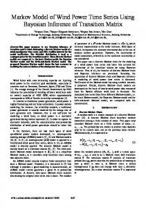
The PV-MC method includes three stages. In the first stage, the wind power state is obtained based on the reformed transition matrix, whose diagonal elements are forced to zero. The state persistence character is not considered in this stage. In the second stage, the wind power state obtained from stage 1 is modified by the distribution of the duration time. In the third stage, the wind power state is converted to a numerical value by using the variation character. State transition, duration time and variation characteristics can be considered in the PC-MC method. The basic flow of using the PV-MC method to generate wind power time series is shown in Figure 1. Step 1. Divide the state of the original wind power time series according to the definition of the wind power state (1), supposing that the total number of states is N (excluding state 0). Step 2. Reform the state transition matrix P. Generate wind power state series P1 based on the reformed state transition matrix using the MCMC method [14]. Step 3. Determine the parameters of the inverse Gaussian distribution function for the duration time of each wind power state based on the Maximum-Likelihood method [28], denoted as (fG)n (n=0, 1, 2,…, N). Step 4. Generate wind power state series P2 by modifying P1 to satisfy the inverse Gaussian distribution function (fG)n (n=0, 1, 2,…, N) of every state. Step 5. Determine the parameters of the t location-scale distribution function for the variation of the original wind power time series based on the Maximum-Likelihood method [28], denoted as ft. Step 6. Generate wind power time series P3 by adding the variations to P2. The variations satisfy ft. After performing the above steps, the new wind power time series, P3, is formed to satisfy the persistence and variation characteristics of the original wind power time series. 3.2
The generation of wind power state series P1
3.2.1 Reforming the state transition matrix P The state transition matrix referred to above contains the transition probabilities of the various states. The matrix cannot consider the duration time character directly, which may lead the duration time of a state when generating the time series to be significantly longer than it should be. To
Li J H, et al.
Sci China Tech Sci
Figure 1
The basic flow of the PV-MC method.
improve this shortcoming, the PV-MC method adjusts the diagonal elements of the state transition matrix by employing the duration time characteristic of the wind power time series. Step 1. Set the values of all diagonal elements of P to 0. Step 2. Recalculate the values of the non-diagonal elements. The new values of the non-diagonal elements equal the ratio of the original value of the non-diagonal elements and the sum of all non-diagonal elements, shown by (8). 0, pkj pkj
k j, N
j 1, j k
pkj ,
k j.
(8)
tion matrix P of the Brazos wind farm, and Figure 2(b) depicts the corresponding reformed state transition matrix P′. Based on the new state change matrix P′, this paper utilises the MCMC method [14] to generate wind power time series P1. 3.2.2 The generation of P1 by MCMC The procedures used to generate P1 are as follows. Step 1. Use state transition matrix P′ to generate the cumulative state transition matrix Pcum as (10). The matrix Pcum is formed by (11). As can be seen from (11), all elements of the 1st column of Pcum are zero, and the maximum value of l should be N+1 to reach j=N. As a result, the dimension of Pcum is (N+1)×(N+2).
Then, the reformed state transition matrix P′ is formed as (9). 0 p10 P pN 0
p01 0
pN 1
p0 N p1N . 0
Pcum
(9)
Figure 2(a) presents the 15-min time interval state transi-
Figure 2
2479
December (2014) Vol.57 No.12
pcum ,00 pcum ,10 p cum , N 0
pcum , kl
pcum ,01 pcum ,11
pcum, N 1
0, l 1 pkj , j 1
pcum ,0( N 1) pcum ,1( N 1) , pcum , N ( N +1)
(10)
l 0, 0 l N 1.
The 15-min state transition matrix of the Brazos wind farm. (a) State transition matrix P; (b) state transition matrix P′.
(11)
2480
Li J H, et al.
Sci China Tech Sci
Step 2. Randomly generate an integer in the range of [0, N] as the initial state of the generated wind power time series; denote this state as d. For example, d=1. Step 3. Randomly generate a number u in the range of [0, 1]. For example, u=0.2. Step 4. Compare u with the dth row elements (the row number is the current state of the wind power time series) of the matrix Pcum. If u is in the range of (pcum de, pcum de+1], then the next state of the wind power time series is e. For example, if d=1, u=0.2 and (pcum 12, pcum 13]=(0.19, 0.22], then the next state of the wind power is e=2. Step 5. If the length of the generated wind power state series meets the requirements, then terminate the simulation; otherwise, return to step 3, and continue with the current state, e. Through the above steps, we can generate a wind power state series P1 that satisfies the Markov state transition condition. It should be noted that P1 is generated based on the state transition matrix P′, whose diagonal elements are 0; this method ignores the persistence character of a state. The persistence character of a state is reconsidered by the wind power duration time character in Section 3.3. 3.3
December (2014) Vol.57 No.12
pre-set number is 15, then the simulation is terminated, and P2=1, 1, 1, 2, 1, 3, 5, 6, 7, 7, 3, 4, 5, 7, 8; else, if the present number is 20, then return to step 2 to determine the state duration of 2. Based on above steps, the series P2 is formed to satisfy both the state transition and duration time characteristics. 3.4
Each element in series P2 is a state representing a range of wind power values, not an exact value. Now, we form wind power time series P3 by superposing the variation on P2 and converting the state to an exact wind power value. Suppose the length of series P2 (the total number of elements) is K; the procedure is detailed as follows. Step 1. Generate a random number set Q{Qj, j=1, 2, 3, …, KQ} that satisfies the t location-scale distribution ft of the original wind power variation. Generally, KQ is significantly larger than the length K of series P2; in this paper, we set KQ=10K. Step 2. Determine the value of the first element. Suppose that the state of the first element is s1. According to the definition of state (1), the value range of s1 is PE PE N * ( s1 1), N * s1 .
The generation of wind power state series P2
The purpose of this part is to add the duration time of each state to series P1 according to the inverse Gaussian distribution function. The procedures are detailed as follows. Step 1. Randomly generate integer sets of the duration time for each state. Taking the nth state as an example, generate a random integer set Ln{lni, i=1,…, KLn} whose distribution satisfies the inverse Gaussian distribution function (fG)n, where KLn is the element number of Ln. Step 2. Proceed through the wind power time series P1 to determine the duration time of each state element by Ln{lni, i=1,…, KLn}. Suppose that the state of the current element in P1 is n; then, the duration time of state n in P1 is determined by following two steps. First, randomly extract an element x1 from Ln (do not put x1 back into Ln, that is, the number of elements in the set is reduced by one), where x1 is regarded as the duration time of state n. Second, replace the current element (state n) in P1 with x1 elements, all with values of n, to form a new series, known as P2′. For example, suppose P1=1, 2, 1, 3, 5, 6, 7, 7, 3, 4, 5, 7, 8, 9 with x1=3; the current element in P1 is the first element, and its state is 1. Then, the new series P2′=1, 1, 1, 2, 1, 3, 5, 6, 7, 7, 3, 4, 5, 7, 8, 9. Step 3. Count the number of elements in series P2′. If the length of P2′ is less than the preset number, then return to step 2 and determine the state duration time of the next state in P1. Otherwise, terminate the simulation, and set P2 equal to the front elements of P2′ with the presented length. For example, now the number of elements in P2′ is 16. If the
The generation of wind power time series P3
(12)
Randomly extract a number x2 (do not return x2) in the range of (12) as the first value element of series P3. Step 3. Determine the value of each element i (1K. Through the above steps, the final series P3, which satisfies the persistence and variation characteristics of wind power, is obtained.
4 4.1
Simulation results Description of the simulation
The data analysed are field-measured wind power output data from 25 wind farms located across the globe. An illustration of original wind power data is provided in Table 2. By dividing the original wind power time series into 11
Li J H, et al.
Sci China Tech Sci
December (2014) Vol.57 No.12
2481
and 21 states, including state 0, we use the 1st order MCMC method, 3rd order MCMC method and PV-MC method to generate respective wind power time series of the same length for the 25 wind farms. In all the figures in this paper, PVMC11 (1), MCMC11 (1) and MCMC11 (3) stand for PVMC method, 1st order MCMC method and 3rd order MCMC method of 11 states, respectively. Accordingly, PVMC21 (1), MCMC21 (1) and MCMC21 (3) stand for PVMC method, 1st order MCMC method and 3rd order MCMC method of 21 states, respectively.
the wind power time series in low output based on the MCMC method is longer than that of the original wind power time series. Additionally, the volatility of the wind power time series of the MCMC method is significantly wider than that of the original wind power time series. However, the results based on the PV-MC method, as presented in Figure 3(d), can improve these shortcomings.
4.2 Simulation results of the wind power time series
Generally, the statistical characteristics of time series mainly include the mean value, variance (or standard deviation), kurtosis, skewness, PDF and ACC.
The England wind farm data are used to demonstrate the results generated for each phase using the proposed PV-MC method. First, a state transition series P1, determined by the off-diagonal elements in the transition matrix, is formed, as in Figure 3(b). Second, the duration time distribution is used to sample the duration time for each state, and a wind power time state series P2 is preliminarily generated, as in Figure 3(c). Third, the variation distribution of the wind power is applied to determine the actual power value in each state to form P3, as in Figure 3(d). Figures 3(a) and (e) are the original wind power time series and that generated by the MCMC, respectively. Compared with Figures 3(a) and (e), the duration time of
4.3 Statistical characteristic analysis of the wind power time series
4.3.1 The mean, standard deviation, kurtosis and skewness The error of the mean value, the standard deviation, skewness and kurtosis between original series and the generated series are shown in Figure 4. The error is
abs ( z g z ),
(14)
where zg is the results of the generated series, and z is the results of the original series. In Figure 4, it can be seen that for the 25 wind farms, the
Figure 3 Comparisons of the wind power time series generated using the MCMC and PV-MC methods with the original series of wind power, based on the data from England (a sample of 15000 min). (a) The original wind power series; (b) the wind power time series of P1; (c) the wind power time series of P2; (d) the wind power time series of P3; (e) the wind power time series generated using the MCMC method.
2482
Li J H, et al.
Sci China Tech Sci
December (2014) Vol.57 No.12
Figure 4 Comparisons of the mean, standard deviation, kurtosis and skewness errors. (a) Comparison of the mean errors; (b) comparison of the standard deviation errors; (c) comparison of the kurtosis errors; (d) comparison of the skewness errors.
errors of the three methods are almost the same. All the three methods have good performance on capturing the base characteristics of mean, standard deviation, kurtosis and skewness. It can be seen from Figure 4 that their mean value error are less than 0.1, standard error are less than 0.08, kurtosis error are less than 0.6 and skewness are less than 0.2. As for the choice of state number, there are not significant differences between 11 states and 21 states division. 4.3.2 PDF The PDF describes the distribution of the random variable. In order to compare the probability distribution error of the
three methods, the quantile-quantile (Q-Q) values of the time series simulated from the methods are plotted against those from the original measurement data as shown in Figures 5(a)–(c). The Q-Q plot offers the advantage of giving more qualitative information and enables highlighting the goodness-of-fit of the simulated distributions on some important parts of the distribution such as the tails which account for extremes events. If the generated time series and the original one are from the same probability distribution, then the Q-Q plot follows a straight line with a unit slope (the dash line in the figure. Figure 5 shows the Q-Q plot of wind farm
Li J H, et al.
Sci China Tech Sci
2483
December (2014) Vol.57 No.12
Figure 5 Comparisons of quantile-quantile (Q-Q) plots. (a) Comparison of Q-Q plot of No.2 wind farm; (b) comparison of Q-Q plot of No.15 wind farm; (c) comparison of Q-Q plot of No.18 wind farm.
2 (Figure 5(a)), wind farm 15 (Figure 5(b)) and wind farm 18 (Figure 5(c)). It is observed from Figure 5(a) that all the three methods fit well for quantiles less than 200 MW, but for wind power larger than 200 MW, the 1st order MCMC method and 3rd order MCMC method fit a little poorer. In Figure 5(b), the 1st order MCMC method deviates from the straight line and gives relatively worst fit in probability distribution among three methods. All the three methods give the best fit in Figure 5(c). This observation indicates that the PVMC method is favoured among the three methods. 4.3.3 ACC The ACC describes the autocorrelation property of a time series. For larger ACC values, the autocorrelation of the time series is stronger. The maximum value of the ACC is 1. The ACC of a time series (z1,…,zn) about the time shift k is calculated by (15). ACC k
cov( zt , zt k ) var( zt ) var( zt k )
,
(k 0, 1, 2,). (15)
In (15), cov and var represent the calculations for the convolution and variance, respectively. Additionally, zt represents the time series (z1,…,zn-k), and zt+k represents the time series (z1+k,…, zn). To compare the two methods more clearly, we adopt the residual sum of squares (RSS) [19] of the ACC curve as the contrasting parameters. RSS z g z . 2
(16)
In (16), zg is the value of the generated series, and z is the value of the original series. The results are shown in Figure 6. The 1st order MCMC method has higher RSS error than others. The performances of PVMC and 3rd order MCMC are close in 21 states division while 3rd order MCMC method is better than PVMC in the 11 states division. As a whole, the 3rd order MCMC method possesses the best ACC characters and the 1st order MCMC method is worst. PVMC is between them. 4.4 Time domain characteristic analysis of wind power series 4.4.1 The distribution of the wind power duration time The studies presented above demonstrate that the wind power duration time follows an inverse Gaussian distribution. Verification of the characteristic is performed by a comparison of the error of the fitted parameters. The error is calculated by the (17), denoted as DT. The duration time characteristic with lower value of DT is the better. The compared results are shown in Figure 7. NQ
DT
1 N
N
Tgi, j Toi, j
j
NQ
i
2
,
(17)
where N is the state number, Ti,j is the ith quantile of the duration time series of jth state, NQ is the number of quantiles, subscript g denotes the generated wind power series while o denotes the original wind power series. Ti,j is calcu-
2484
Li J H, et al.
Figure 6
Sci China Tech Sci
Comparisons of the ACCs of the RSSs. (a) Comparisons of 11 states; (b) comparisons of 21 states.
lated by linear interpolation between closest ranks (Hazen, 1914) introduced in [29]. A comparison of the errors is shown in Figure 7. As can be seen from the figure, the PVMC gives lowest DT value in all the 25 wind farms no matter in division of 11 states or 21 states. It indicates that the PVMC method has the best performance on possessing the duration time characteristic among the three methods. The 3rd order MCMC method does not give much better performance than 1st order MCMC method in Figure 7, because the duration time characteristic is not considered in MCMC method. Besides, the results of 21 states division are better than that of 11 states in preserving the duration time feature. 4.4.2 The transition matrix of the wind power state The characteristic of the wind power state transition is mainly reflected in the state transition matrices; however, such matrices are difficult to compare directly. Therefore, the task requires an index for ease of comparison. In light of this, the Frobenius norm (F-norm) of the error matrix between the state transition matrices of the generated and original wind power data is introduced as the index for describing the similarity of the two matrices. F-norm is defined in (18). For smaller values of F-norm, the wind power state transition characteristic of the generated time series is closer to the original one. 1/ 2
A
Figure 7
F
December (2014) Vol.57 No.12
n n 2 aij i 1 j 1
1/ 2
tr( AH A)
,
(18)
where A ( aij ) C nn , C is the n-dimensional real matrix, and aij is the difference between state transition matrix elements of the generated series and the original series. A comparison of the F-norm errors yielded using the three methods is shown in Figure 8. The errors of F-norms of the 1st order transition matrix based on the three methods are similar. While for the 2nd and 3rd order transition matrix, the 3rd order MCMC method is much better than the 1st order MCMC method and PVMC method. Seen from Figure 8, the error of 2nd state transition matrix F-norm of 11 states division is smaller than that of 21 states, which indicates that the results of 21 states division are not always better than that of 11 states in possessing the state transition characteristic. 4.4.3 The variation distribution of the wind power The studies above show that the wind power variation is t location-scale distribution. Hence, verification of the characteristic is performed by a comparison of the errors of the fitted parameters. The error is calculated by the (17), denoted as VA. The compared results are shown in Figure 9. Comparisons of the errors are shown in Figure 9. As can be seen from the figure, the PVMC gives lowest VA value in all the 25 wind farms no matter in division of 11 states or 21 states. It indicates that the PVMC method has the best performance on possessing the variation characteristic among the three methods. The 3rd order MCMC method doesn’t give better performance than 1st MCMC method in Figure 9, because the variation characteristic is not considered in
Comparisons of the goodness-of-fit of the wind power duration time distribution. (a) Comparisons of 11 states; (b) comparisons of 21 states.
Li J H, et al.
Sci China Tech Sci
December (2014) Vol.57 No.12
2485
Figure 8 Comparisons of the wind power state transition matrix F-norm values. (a) Comparison of the F-norm error of 1st order state transition; (b) comparison of the F-norm error of 2nd order state transition matrix; (c) comparison of the F-norm error of 3rd order state transition matrix.
Figure 9
Comparisons of the goodness-of-fit of the wind power variation characteristic. (a) Comparisons of 11 states; (b) comparisons of 21 states.
MCMC method. Besides, the results of 21 states are better than that of 11 states in preserving variation feature.
5 Conclusions In response to the disadvantages of the MCMC method in terms of generating wind power time series, this paper proposed an innovative method, namely, the PV-MC method,
which is based on analysing the persistence and variation characteristics of wind power time series. The results of various comparisons of the characteristics of the wind power series generated using both methods relative to the original data for 25 wind farms show that the PV-MC method can generate a significant number of wind power series and that these series are closer to the duration time and variation distribution characteristics of the original series, which is in contrast to the results based on the MCMC method, assum-
2486
Li J H, et al.
Sci China Tech Sci
ing the other characteristics remain unchanged greatly. The presented PV-MC method provides support for various problems, such as large-scale wind power system reliability evaluation and probabilistic load flow calculation, among others. This work was supported by the National Natural Science Foundation of China (Grant No. 51377027), the National Basic Research Program of China (“973” Project) (Grant No. 2012CB215104) and ABB (China) Ltd.
1 2
3
4
5
6
7
8
9 10 11
12
Liu J Z, Liu Y, Zeng D L, et al. Optimal short-term load dispatch strategy in wind farm. Sci China Tech Sci, 2012, 55: 1140–1145 Miao W W, Jia H J, Wang D, et al. Active power regulation of wind power systems through demand response. Sci China Tech Sci, 2012, 55: 1667–1676 Abbey C and Joós G. A stochastic optimization approach to rating of energy storage systems in wind-diesel isolated grids. IEEE Trans Power Syst, 2009, 24: 418–426 García-González J, de la Muela R M R, Santos L M, et al. Stochastic joint optimization of wind generation and pumped-storage units in an electricity market. IEEE Trans Power Syst, 2008, 23: 460–468 Billinton R, Wangdee W. Reliability-based transmission reinforcement planning associated with large-scale wind farms. IEEE Trans Power Syst, 2007, 22: 34–41 Billinton R, Chen H, Ghajar R. Time series models for reliability evaluation of power systems including wind energy. Microelectron Reliab, 1996, 36: 1253–1261 Lojowska A, Kurowicka D, Papaefthymiou G, et al. Advantages of ARMA-GARCH wind speed time series modeling. In: 2010 IEEE 11th International Conference on Probabilistic Methods Applied to Power Systems. Singapore, 2010. 83–88 Shamshad A, Bawadi M A, Wan Hussin W M A, et al. First and second order Markov chain models for synthetic generation of wind speed time series. Energy, 2005, 30: 693–708 Kitagawa T, Nomura T. A wavelet-based method to generate artificial wind variation data. J Wind Eng Ind Aerod, 2003, 91: 943–964 Box G and Jenkins G, Time Series Analysis–Forecasting and Control. San Francisco, CA: Holden-Day, 1976 Hill D C, McMillan D, Bell K R W, et al. Application of autoregressive models to U.K. wind speed data for power system impact studies. IEEE Trans Sustain Ener, 2012, 3: 134–141 Chen P, Pedersen T, Bak-Jensen B, et al. ARIMA-Based time series model of stochastic wind power generation. IEEE Trans Power Syst, 2010, 25: 667–676
December (2014) Vol.57 No.12
13
14 15
16
17
18
19
20
21
22 23
24 25 26 27
28 29
Murugesan S, Zhang J, Vittal V. Finite state Markov chain model for wind generation forecast: a data-driven spatiotemporal approach. In: 2012 IEEE PES Innovative Smart Grid Technologies (ISGT). Washington DC, 2012. 1–8 Papaefthymiou G, Klőckl B. MCMC for wind power simulation. IEEE Trans Energy Convers, 2008, 23: 234–240 Abdel-Karim N, Small M, Ilić M. Short term wind speed prediction by finite and infinite impulse response filters: A state space model representation using discrete Markov process. In: 2009 IEEE Vucharest Power Tech. Bucharest, 2009. 1–8 Sturt A, Strbac G. Time-series modelling for the aggregated great Britain wind output circa 2030. Iet Renew Power Gen, 2012, 7: 36– 44 Woods M J, Russell C J, Davy R J, et al. Simulation of wind power at several locations using a measured Time-Series of wind speed. IEEE Trans. Power Syst, 2013, 28: 219–226 Sun H S, Li J M, Li J H, et al. An investigation of the persistence property of wind power time series. Sci China Tech Sci, 2014, 57: 1578–1587 Lin W X, Wen J Y, Cheng S J, et al. An investigation on the activepower variations of wind farms. IEEE Trans Ind Appl, 2012, 48: 1087–1094 Villegas C, Paula G A, Leiva V. Birnbaum-Saunders mixed models for censored reliability data analysis. IEEE Trans Rel, 2011, 60: 319– 327 Balakrishnan N, Lin C T, Chan P S. A comparison of two simple prediction intervals for exponential distribution. IEEE Trans Rel, 2005, 54: 27–33 Chhikara R S, Folks J L. The Inverse Gaussian Distribution: Theory, Methodology, and Applications. M. Dekker, 1989 Buzaianu E M, Chen P, Wu T J. Subset selection procedures to identify electromagnetic fields following lognormal distributions. Iet Radar Sonar Nav, 2011, 5: 458–465 Kirby B, Hirst E. Generator response to intrahour load fluctuations. IEEE Trans Power Syst, 1998, 13: 1373–1378 Hirst E, Kirby B. Defining intra-and interhour load swings. IEEE Trans Power Syst, 1998, 13: 1379–1385 Chen Z, Ni W D, Li Z. Preliminary study on wind power characteristics. Acta Energi, 2011, 32: 210–215 Wu T, Ai X M, L W X, et al. Markov chain Monte Carlo method for the modelling of wind power time series. In: Innovative Smart Grid Technologies-Asia (ISGT Asia). Tianjin, 2012. 1–6 Papoulis A, Pillai S U. Probability, Random Variables and Stochastic Processes, 4th ed. New York, NY: McGraw-Hill, 2002. 260–262 Hyndman R J, Yanan F. Sample quantiles in statistical packages. Am Stat, 1996, 50: 361–365