Yuen-Hsien Tseng, " Generic Title Labeling for Clustered Documents", Expert Systems With Applications, Vol. 37, No. 3, 15 March 2010, pp. 2247-2254.
Generic Title Labeling for Clustered Documents Yuen-Hsien Tseng National Taiwan Normal University, No. 162, Sec, 1, Heping East Road, Taipei, Taiwan, R.O.C., 106
[email protected]
Abstract Document clustering is a powerful technique to detect topics and their relations for information browsing, analysis, and organization. However, clustered documents require post-assignment of descriptive titles to help users interpret the results. Existing techniques often assign labels to clusters based only on the terms that the clustered documents contain, which may not be sufficient for some applications. To solve this problem, a cluster labeling algorithm for creating generic titles, based on external resources such as WordNet, is proposed. Our method first extracts category-specific terms as cluster descriptors. These descriptors are then mapped to generic terms based on a hypernym search algorithm. The proposed method has been evaluated on a patent document collection and a subset of the Reuters-21578 collection. Experimental results revealed that our method performs as anticipated. Real-case applications of these generic terms show promising in assisting humans in interpreting the clustered topics. Our method is general enough such that it can be easily extended to use other hierarchical resources for adaptable label generation.
Keywords: Hypernym search, clustering labeling, WordNet, correlation coefficient, topic identification.
1. Introduction Document clustering is a powerful text mining technique to detect topics and their relations for information browsing, analysis, and organization. However, unlike document categorization where a set of labels or terms is predefined for each category, the documents sets partitioned, either hierarchically or non-hierarchically, by a clustering algorithm have virtually no such predefined labels for convenient recognition of the content of each set. Each of them requires post-assignment of a concise and descriptive title to help analysts to interpret the result. Although good clustering algorithms are widely available, good solutions for labeling the clustered results to meet analysts’ needs are rare. Most existing work selects the title words from the terms contained in the clustered documents themselves. Although this is justifiable, this may not be sufficient. It would be desirable to further suggest generic topic terms for ease of analysis, especially in the applications where documents cover a wide range of domain knowledge. Examples of this need are often found in topic analysis for patent or scientific publications [1-3]. In this work, we attempt to automatically create generic labels which do not necessarily exist in the clustered documents for easier cluster interpretation. As an example, if the documents in a cluster were talking about tables, chairs, and beds, then a title labeled “furniture” would be perfect for this cluster, especially when this hypernym does not occur in it (or occurs rarely). This kind of problem was often solved by human experts, such as those in [4-5], where cluster titles were given manually. To make our automatic approach feasible, external resources such as WordNet or other hierarchical knowledge structures are used. Our method first selects content-indicative terms for each cluster. A proposed hypernym search algorithm is then applied to map these terms into its generic title. The rest of the paper is organized as follows: Section 2 reviews some related work. Section 3 introduces our method for content-indicative term extraction. Section 4 describes the hypernym search algorithm based on WordNet. Section 5 details the experiments that evaluate our method. Section 6 discusses the results and suggests possible improvement. Section 7 concludes this work and shows its implications.
2. Related Work Labeling a clustered set of documents is an inevitable task in text clustering applications. Automatic labeling methods mainly rely on extracting significant terms from clustered documents, where the term significance can be calculated very differently from clustering algorithms to algorithms. For example, in the vector space model, where clusters are represented as weighted sums or centroids of the document vectors, terms with heaviest weights in the cluster vectors are extracted as the cluster labels. In [6-7], the term weight in a document vector is the normalized term frequency (TF), while in [8], it is a version of the TF multiplied by IDF (Inverse Document Frequency) weighting scheme. As to its effectiveness, the authors in [9] pointed out (although without experiments) that the simple centroid-based approach outperformed the probabilistic odds scheme which computes the ratio of the conditional probability of a term appearing in a cluster over the sum of the conditional probabilities of the term in other clusters. The authors in [10] proposed a linear model to combined at least 10 features including TF, TFxIDF, and statistical information from the surrounding clusters (sibling clusters or parent cluster) to rank the terms in the clustered documents. However, it requires human labeled titles to train the model for setting optimal model parameters.
2
In the Self-Organization Map (SOM) method [11], where clusters are organized in a 2-D map, the label of a cluster is the term having the highest goodness measure. This goodness measure is the square of the relative term frequency in the cluster normalized by the sum of the relative term frequencies in other distant clusters. In an application to group terms for detecting events over time [12], the cluster title consists of the highest ranked named entity followed by the highest ranked noun phrase. The ranks of these terms were obtained by sorting the maximum chi-square values of the terms occurring in a time interval. In clustering web search results, the longest phrases occurred in most documents in a cluster were used as its title [13]. In other related fields, such as document summarization and translation, there were tasks in the Document Understanding Conference (DUC) [14] to generate very short summaries. These short 10-words summaries have the potential to serve as cluster titles. However, most participants use extraction-based methods [15]. Even though there were studies that generate document titles not from the document themselves, a large corpus of documents with human-assigned titles is required to train the “translation model” so as to map document words into human-assigned titles [16]. Besides, these summaries tend to be event-descriptive rather than topicindicative for a set of documents. As can be seen, despite there are various techniques to label a set of documents, there are few studies that attempted to deal with the problem that we propose here.
3. Cluster Descriptor Selection The methods to extract cluster descriptors in the above-mentioned studies are mostly related to their clustering algorithms. In our application, we would like to have a general approach that is independent of the clustering process. To this end, we seek solutions from text categorization where selecting the best content-revealing or category-predictive features has been widely studied. Yang et al [17] had compared five different methods for selecting category-specific terms. They found that chi-square is among the best that lead to highest categorization performance. The chi-square method computes the relatedness of term T with respect to category C in the manner:
χ 2 (T , C ) =
(TP × TN - FN × FP)2 . (TP + FN)(FP + TN)(TP + FP)(FN + TN)
(1)
where TP (True Positive), FP (False Positive), FN (False Negative), and TN (True Negative) denote the number of documents that belong or not belong to C while containing or not containing T, respectively. With content terms (in the same cluster) sorted by their chi-square values in descending order, top-ranked terms can be selected as the cluster descriptors. However, chi-square does not distinguish negatively related terms from positively ones. A remedy to this problem is the use of the correlation coefficient (CC), which is just the square root of the chi-square: Co(T , C ) =
(TP × TN - FN × FP) . (TP + FN)(FP + TN)(TP + FP)(FN + TN)
(2)
As pointed out by Ng et al [18], correlation coefficient selects exactly those words that are highly indicative of membership in a category, whereas the chi-square method not only picks out this set of terms but also those terms that are indicative of non-membership in that category. This is especially true when the selected terms are in small number. As an example, in a small real-world collection of 116 short documents (containing only the titles) with only two exclusive categories: construction vs. non-construction in civil engineering tasks, some of the best and worst terms that are computed by both methods are shown in Table 1. As can be seen, 3
“engineering” is a lowest-ranked term (-0.7880) based on correlation coefficient in the non-construction category, while it is a top-ranked term in both categories based on chi-square (0.6210 is the square of -0.7880). Therefore, instead of chi-square, correlation coefficient is used as our basic descriptor selection method. Table 1. Some best and worst terms computed by chi-square and correlation coefficient in a collection with two exclusive categories. Chi-square Construction Non-Construction engineering improvement … kitchen update
Correlation Coefficient Construction Non-Construction
0.6210 engineering 0.6210 engineering 0.1004 improvement 0.1004 improvement … 0.0009 kitchen 0.0009 communiqué 0.0006 update 0.0006 equipment
0.7880 0.3169
equipment procurement
0.2854 0.2231
-0.2062 improvement -0.3169 -0.2854 engineering -0.7880
A further analysis of the correlation coefficient method reveals that it may be effective only for the case where the collection to be clustered contains large number of short documents. For the collections containing long documents, it tends to select category-specific terms that are too specific due to the ignorance of the term frequency in each document (i.e., TF). Therefore, we choose only those terms whose document frequency in a cluster exceeds a ratio r of the number of documents in that cluster. We denote this revised method as CCr, where r is a tunable parameter and is 0.5 in our implementation. Another remedy is to multiply the term’s CC with its total term frequency in the cluster (TFC), denoted as CCxTFC, where TFC is the sum of a term’s TF over all documents in the cluster.
4. Generic Title Generation The cluster descriptors generated in the above may not be topic-indicative enough to well summarize the contents of the clusters (e.g., see the examples in later sections). One might need to map the identified clusters into some predefined categories for supporting other data mining tasks (e.g. [19]). If the categories have existing data for training, this mapping can be recast into a standard text categorization problem, to which many solutions can be applied. Another need arises from the situation that there is no suitable classification system at hand, but some generic labels are still desired for quick interpretations. This case is often solved by human experts, where cluster titles are given manually. Below we propose an automatic solution by use of an extra resource, i.e., WordNet. WordNet is a digital lexical reference system [20]. English nouns, verbs, adjectives and adverbs are organized into synonym sets. Different relations, such as hypernym, hyponym, meronym, or holonym, are defined to link the synonym sets. With these structures, one can look up in WordNet all the hypernyms of a set of given terms and then choose the best among them as the generic title with some heuristic rules. Since the hypernyms were organized hierarchically, the higher is the level, the more generic are the hypernyms. To maintain the specificity of the set of terms while revealing their general topics, the heuristics have to choose as low-level common hypernyms as possible. When there are multiple choices, ranks should be given to order the hypernyms in priority. In our implementation, we look up for each given term all its hypernyms alone the path up to the root in the hierarchical tree. The number of occurrence (f) and the depth in the hierarchy (d) of an encountered hypernym are recorded. With the root being given a depth value of 0, a weight proportional to the normalized f and d is calculated for each hypernym as follows:
4
weight (hypernym) =
⎛ ⎞ f 1 × 2 × ⎜⎜ − 0.5 ⎟⎟ . −c×d nt 1 + exp ⎝ ⎠
(3)
where nt is the number of given terms to normalize the occurrence f to a value ranges from 0 to 1 and c (0.125 in our implementation) is a constant to control the steepness of the sigmoid function 1/(1+exp(-c x d)) whose value approaches 1 (-1) for large positive (negative) d. Since the depth d only takes on non-negative value, the actual range of the sigmoid is from 0.5 to 1. It is thus subtracted with 0.5 and then multiplied by 2 to map the value of d into the normalized range: 0 to 1. Note that a term having no hypernym or not in WordNet is omitted from being counted in nt. Also note that a term can have multiple hypernyms and thus multiple paths to the root. A hypernym is counted only once for each given term, no matter how many times the multiple paths of this term pass this hypernym. This weight is finally used to sort the hypernyms in decreasing order to suggest priority. In the example mentioned at the beginning, where the 3 terms were given: table, chair, and bed, their hypernym: “furniture” did result from the above calculation with a highest weight 0.3584 based on WordNet version 1.6, as shown in Figure 1. The other two hypernyms are “geology” and “tableland”, with weights: 0.1633 and 0.1372, respectively. entity
object Natural_object act
artifact
geology
location
activity group; grouping
elevation
instrumentation occupation
arrangement
highland
tabular array
tableland
furnishings job
furniture
position
seat table
region
device
layer
instrument instr. of exec.
Nat. depression
stratum
bed
chair
Figure 1. The hypernym structure of the three words based on WordNet.
5. Experiments In this section, we evaluate the proposed method by two collections having opposite characteristics, one contains long documents, the other contains short but relatively many documents. 5.1 Document Collections The first collection contains 612 patent documents downloaded from the USPTO’s website [21] with “National Science Council” (NSC) as the search term in the assignee field. NSC is the major government agency that sponsors research activities in Taiwan. Institutes, universities, or research centers, public or private, can apply research fundings from NSC. Once the research results have been used to apply for US patents, the intellectual property rights belong to NSC. In other words, NSC becomes the assignee of the patents. However, this policy 5
has been changed since year 2000 so that the number of NSC patents per year declines since then. Due to this background, these documents constitute a knowledge-diversified collection with relative long texts (about 2000 words per document) describing various advanced technical details. Analysis of the topics in this collection becomes a non-trivial task as very few analysts know of such diversified technologies and fields. Although each patent has pre-assigned International Patent Classification (IPC) or US Patent Classification (UPC) codes, many of these labels are either too general or too specific such that they do not fit the intended knowledge structures for topic interpretation. Therefore, using them alone does not meet the requirement of the intended analysis. As such, computer-suggested labels play important roles in helping humans understand this collection. This work is in fact motivated by such a need. The other collection is a subset of the widely used Reuters-21578 collection for text categorization. It contains brief stories (about 133 words per story) in the financial domain. Each document was assigned at least one category to denote its topics and there are a total of 90 categories based on Yang’s preprocessing rules [22]. In this work we used the largest 10 categories of them to evaluate our method.
5.2 Document Clustering Since it is hard to have a consensus on the number of clusters to best organize the NSC collection, we clustered it using different options and parameters to get various views on it. Specifically, we analyzed the collection based on document clustering and term clustering as well. The 612 US patent documents were parsed, filtered, segmented, and summarized. Structured information in the documents such as assignees, inventors, and IPC codes were removed. The remaining textual parts were segmented into several main sections (Abstract, Claims, Field of the Invention, Background of the Invention, Summary of the Invention, and Detailed Descriptions) based on the regularity of the patent document style [23]. Since these sections vary drastically in length, they were summarized using extraction-based methods [24] to select at most 6 best sentences from each section. They were then concatenated to yield the document surrogates for key term extraction, term co-occurrence analysis, indexing, and clustering. These document surrogates did not include the Claims section due to its legal-oriented contents. From the document surrogates, 19,343 key terms (terms occur at least twice in a document) were extracted. They were used in the term co-occurrence analysis to see which terms are often co-occurred with each other in the same sentence [25]. Only 2714 of the key terms occur in at least two documents and have at least one term co-occurred with them. These 2714 terms were clustered by a complete-link method into 353 small-size clusters, based on how many co-occurred terms they share. These clusters were then repeatedly clustered, again based on the common co-occurred terms (co-words), into 101 medium-size clusters, then into 33 large-size clusters, and finally into 10 topic clusters. The reason that we performed this multi-stage clustering is due to the fact that even we set the lowest threshold, we could not obtain as low as 10 clusters in a single step. The 353 small-size clusters are actually obtained with the similarity threshold set to 0.0. In other words, among the 2714 terms, no two terms in different small-size clusters share the same co-words. Through this multi-stage term clustering, the topics of the collection were revealed as the key terms were merged into concepts, which in turn were merged into topics or domains. This approach has the merit that it can be efficiently applied to very large collections due to the fast co-occurrence analysis [25]. As another way for topic analysis, the 612 NSC patents were clustered directly based on their summary surrogates. We call this method document clustering. As with the above term clustering, they were first clustered into 91 topics, which in turn were grouped into 21 sub-domains, from which 6 major domains were found. For a collection, the main concern to choose between direct document clustering and the indirect term clustering for topic identification lies in the computation feasibility. Because the clustering algorithm itself 6
requires high order of computation complexity, direct document clustering can only apply to a limited number of documents, while the above term clustering can normally apply to a larger number of documents with several orders of magnitudes (by limiting the number of terms). In this NSC collection, both clustering methods can be applied since it is relatively small. The advantage is that we can observe different topic sets, which are often complimentary to each other. For the second collection, we did not cluster the Reuters collection since it already has been organized by its predefined labels. These labels were used to compare with our cluster titles.
5.3 Evaluation of Descriptor Selection For comparison, we used three methods to rank cluster terms for descriptor selection, namely TFC, CC0.5, and CCxTFC, as defined in Section 3. These ranking methods were applied to three sets of the clustering results mentioned above. The first is the first-stage document clustering. The second is the second-stage document clustering. The third is the third-stage term clustering based on their co-words. For each cluster, at most 5 best terms were selected as its descriptors. Two master students majored in library science were invited to compare the relative quality of these descriptors under the same clusters. For each ranking method, the number of cases where it has the best title quality over the other methods was counted. Multiple best choices for a cluster are allowed and those cluster descriptors that are hard to assess can be omitted from being considered. The ranking methods are coded in such a way that the assessors do not know which method is used to select the examined descriptors. The assessment results are shown in Table 2. Note hierarchical clustering structures were shown to the assessors. They were free to examine whatever clusters or sub-clusters they were interested in. This is why the numbers of examined clusters differ between them. In spite of this difference, this preliminary experiment shows that cluster descriptors selected by CC0.5 or CCxTFC are favorable by one assessor each, while those generated by TFC are not by either. This is somewhat useful to know, since most past studies use TFC or a variation of it to generate cluster titles, as mentioned in Section 2. Table 2. Comparison of three descriptor selection methods among three cluster sets. Ranking No. of clusters No. of clusters No. of clusters No. of clusters method Assessor that TFC is the that CC0.5 is the that CCxTFC is examined Cluster set best best the best 1 73 5 7% 52 71% 20 27% First-stage doc. clusters 2 19 6 32% 12 63% 13 68% 1 13 0 0% 9 69% 6 46% Second-stage doc. clusters 2 7 1 14% 3 43% 5 71% 1 16 5 31% 12 75% 9 56% Third-stage term clusters 2 10 5 50% 4 40% 8 80%
5.4 Evaluation of Generic Title Generation The proposed title mapping algorithm was applied to the final-stage results of the document clustering and term clustering described above. The first set has 6 clusters and the second has 10. Their best 5 descriptors selected by CCxTFC are shown in the second column of Table 3. The proposed method was compared to a similar tool called InfoMap [26] which is developed by the Computational Semantics Laboratory at Stanford University. This online tool finds a set of taxonomic classes for a list of given words. It seems that WordNet is also used as its reference system, because the output classes are mostly WordNet’s terms. Since no technical details about InfoMap were found on the Web, we cannot implement the InfoMap’s algorithm by ourselves. Therefore, an agent program was written to send the 7
descriptors to InfoMap and collect the results that it returns. Only the top-three candidates from both methods are compared. They are listed in the last two columns in Table 3, with their weights appended. The reasonable classes are marked in bold face in the table. As can be seen, the two methods perform similarly. Both achieve a level of 50% accuracy in either set. Table 3. Descriptors and their machine-derived generic titles for the NSC collection ID 1 2 3 4 5 6
1 2 3 4 5 6 7 8 9 10
Cluster’s Descriptors
WordNet
1:substance, matter:0.1853 acid, polymer, catalyst, ether, 2:drug:0.0980 formula 3:chemical compound:0.098 1:object, physical object:0.1244 silicon, layer, transistor, gate, 2:device:0.1211 substrate 3:artifact, artefact:0.1112 1:device:0.1514 plastic, mechanism, plate, rotate, 2:base, bag:0.1155 force 3:cut of beef:0.1155 1:communication:0.1470 output, signal, circuit, input, 2:signal, signaling, sign:0.1211 frequency 3:relation:0.0995 1:substance, matter:0.1483 powder, nickel, electrolyte, steel, 2:metallic element, metal:0.1211 composite 3:instrumentation:0.0980 1:substance, matter:0.1112 gene, protein, cell, acid, expression 2:object, physical object:0.0995 3:chemical compound:0.0980 1:substance, matter:0.1853 resin, group, polymer, compound, 2:chemical compound:0.098 methyl 3:whole:0.0717 1:communication:0.1470 circuit, output, input, signal, voltage 2:signal, signaling, sign:0.1211 3:production:0.0823 1:substance, matter:0.1483 silicon, layer, material, substrate, 2:object, physical object:0.1244 powder 3:artifact, artefact:0.1112 1:artifact, artefact:0.1483 system, edge, signal, type, device 2:communication:0.1470 3:idea, thought:0.0980 1:communication:0.1633 solution, polyaniline, derivative, 2:legal document,:0.1540 acid, aqueous 3:calculation, computation:0.1372 1:device:0.1514 sensor, magnetic, record, calcium, 2:object, physical object:0.1244 phosphate 3:sound/audio recording:0.12 1:structure, construction:0.1225 gene, cell, virus, infection, plant 2:contrivance, dodge:0.1155 3:compartment:0.1029 1:property:0.1112 density, treatment, strength, control, 2:economic policy:0.1020 arrhythmia 3:attribute:0.0995 1:pistol, handgun, side arm:0.1020 force, bear, rod, plate, member 2:unit, social unit:0.0980 3:instrumentation:0.0980 1:artifact, artefact:0.1390 transistor, layer, channel, 2:structure, body structure:0.1225 amorphous, effect 3:semiconductor:0.1029
InfoMap 1:chemical compound:1.25 2:substance, matter:1.062 3:object, physical object:0.484 1:object, physical object:0.528 2:substance, matter:0.500 3:region, part:0.361 1:device:0.361 2:entity, something:0.236 3:chemical process:0.0 1:signal, signaling, sign:1.250 2:communication:1.000 3:abstraction:0.268 1:metallic element, metal:0.500 2:substance, matter:0.333 3:entity, something:0.203 1:entity, something:0.893 2:chemical compound:0.500 3:object, physical object:0.026 1:substance, matter:2.472 2:object, physical object:0.736 3:chemical compound:0.5 1:signal, signaling, sign:1.250 2:communication:1.000 3. round shape:0.000 1:substance, matter:2.250 2:artifact, artefact:0.861 3:object, physical object:0.833 1:instrumentality:1.250 2:communication:0.861 3:artifact, artefact:0.750 1:drug of abuse, street drug:0.000 2:chemical compound:0.0 3:set:0.000 1:device:0.312 2:fact:0.000 3:evidence:0.000 1:entity, something:0.790 2:life form, living thing:0.5 3:room:0.000 1:power, potency:1.250 2:property:0.674 3:condition, status:0.625 1:unit, social unit:1.250 2:causal agent, cause,:0.625 3:organization:0.500 1:anatomical structure:0.500 2:artifact, artefact:0.040 3:validity, validness:0.000
The 10 largest categories in the Reuters collection constitute 6018 news stories. Since they are both short and in a large number in each of these categories, the basic CC method was used to select the cluster descriptors. As can be seen from the third column in Table 4, 8 (those in boldface) out of 10 machine-selected descriptors clearly coincide with the human labels, showing that the effectiveness of the CC method in this collection. When compared to the results made by [27], as shown in Table 5, where mutual information (MI) was used to rank statistically significant features for text categorization, the CC method yields better topical labels than the MI method. 8
As to the generic titles shown in Table 4, about 70% of the cases lead to reasonable results for both the WordNet and the InfoMap methods. It is known that the Reuters labels can be organized hierarchically for further analysis [28]. For example, grain, wheat, and corn can be merged into a more generic category, such as foodstuff. As can be seen from Table 4, this situation was automatically captured by the proposed method. Table 4. Descriptors and their generic titles for the Reuters collection ID
Category
1
earn
2
acq
3
money-fx
4
grain
5
crude
6
trade
7
interest
8
ship
9
wheat
10
corn
Descriptors
WordNet
1:goal:0.2744 NET, QTR, Shr, cts Net, Revs 2:trap:0.2389 3:income:0.2389 1:device:0.1514 acquire, acquisition, stake, 2:stock certificate, stock:0.1386 company, share 3:wedge:0.1386 1:backlog, stockpile:0.0850 currency, money market, 2:airplane maneuver:0.0850 central banks, TheBank, yen 3:marketplace, mart:0.0770 1:seed:0.1848 wheat, grain, tonnes, 2:cereal, cereal grass:0.1848 agriculture, Corn 3:foodstuff, food product:0.182 1:lipid, lipide, lipoid:0.2150 crude oil, bpd, OPEC, mln 2:oil:0.1646 barrels, petroleum 3:fossil fuel:0.1211 1:business:0.0823 trade, tariffs, Trading surplus, 2:UN agency:0.0823 deficit, GATT 3:prevailing wind:0.0823 1:charge:0.1372 rate, money market, bank, 2:airplane maneuver:0.0850 prime, discount 3:allowance, adjustment:0.0850 1:craft:0.2469 ship, vessels, port, Gulf, 2:instrumentation:0.1959 tankers 3:vessel, watercraft:0.1848 1:weight unit:0.1792 wheat, tonnes, grain 2:foodstuff, food product:0.151 agriculture, USDA 3:executive department:0.1386 1:seed:0.1848 corn, maize, tonnes, soybean, 2:cereal, cereal grass:0.1848 grain 3:foodstuff, food product:0.182
InfoMap 1:trap:1.000 2:game equipment:1.000 3:fabric, cloth, textile:1.000 1:asset:0.500 1:medium of exchange, monetary system:0.750 1:weight unit:1.250 2:grain, food grain:1.250 3:cereal, cereal grass:1.250 1:oil:0.750 2:fossil fuel:0.750 3:lipid, lipide, lipoid:0.500 1:liability, financial obligation, indebtedness, pecuniary obligation:0.062 1:charge:0.111 1:craft:0.812 2:physical object:0.456 3:vessel, watercraft:0.361 1:weight unit:1.250 2:foodstuff, food product:0.500 1:cereal, cereal grass:1.250 2:weight unit:1.250 3:foodstuff, food product:0.790
Table 5. Three best words in terms of MI and their categorization break-even precision (BEP) rate of the 10 largest categories of Reuters [27]. Category earn acq money-fx grain crude trade interest ship wheat corn
1st word vs+ shares+ dollar+ wheat+ oil+ trade+ rates+ ships+ wheat+ corn+
2nd word cts+ vsvstonnes+ bpd+ vsrate+ vstonnes+ tonnes+
3rd word loss+ inc+ exchange+ grain+ OPEC+ ctsvsstrike+ wheat+ vs-
BEP 93.5% 76.3% 53.8% 77.8% 73.2% 67.1% 57.0% 64.1% 87.8% 70.3%
6. Discussions The application of our generic title generation algorithm to the NSC patent collection leads to barely 50% of the clusters to have reasonable results. However, this is due to the limit of WordNet in this case. WordNet does not cover all the terms extracted from the patent documents. Also WordNet’s hypernym structures may not reflect 9
the knowledge domains desired for analyzing these patents. On one hand, if the texts of the documents better fit the vocabulary of WordNet, the performance improves, as is the case in the Reuters collection. On the other hand, it is thus anticipated that if a suitable classification system can be found for the document collection to be analyzed, the hypernym search algorithm may lead to more desirable labels. We have tried Google’s directory for the NSC collection, but the categories returned from searching the hypernyms did not meet the intention to analyze the collection. So far we haven’t found any better classification systems that improve the generic titles of the NSC clusters. However, even with the current level of performance using WordNet, this method, as well as the method to select the cluster descriptors, is still helpful, as noted by some NSC analysts. As an example, Figure 2 shows a topic map of the 612 NSC patents. In this figure, each circle denotes an identified topic, the size of the circle denotes the number of patents belonging to the topic, and the number in the circle corresponds to the topic ID. With the Multi-Dimensional Scaling (MDS) method [29] to map these clustered topics in a 2-dimension graph, the relative distance between each topic in the map reflects their relatedness (while the absolute position and orientation of each topic does not matter). Details of the topic titles and their IDs are shown in Table 6. The 6 major domains circled by dashed lines in the figure were those derived from the final-stage document clustering and were labeled by hand with the help of the proposed method.
2. Electronics and Semi-conductors
5. Material
1.Chemistry 4. Communication and computers 3. Generality
6. Biomedicine
Figure 2. A topic map resulted from analyzing the 612 NSC patent documents. Table 6. Final-stage document clusters from the NSC patents. 1: 122 docs. : 0.2013 (acid:174.2, polymer:166.8, catalyst:155.5, ether:142.0, formula:135.9) * 108 docs. : 0.4203 (polymer:226.9, acid:135.7, alkyl:125.2, ether:115.2, formula:110.7) o 69 docs. : 0.5116 (resin:221.0, polymer:177.0, epoxy:175.3, epoxy resin:162.9, acid: 96.7) + ID=131 :26 docs.:0.2211(polymer: 86.1, polyimide: 81.1, aromatic: 45.9, bis: 45.1, ether …) + ID=240 : 43 docs.:0.1896(resin:329.8, acid: 69.9, group: 57.5, polymer: 55.8, monomer: 44.0) o ID=495:39 docs.:0.1385(compound: 38.1, alkyl: 37.5, agent: 36.9, derivative: 33.6, formula …) * ID=650 : 14 docs. : 0.1230(catalyst: 88.3, sulfide: 53.6, iron: 21.2, magnesium: 13.7, selective: 13.1) 2: 140 docs. : 0.4068 (silicon:521.4, layer:452.1, transistor:301.2, gate:250.1, substrate:248.5) * 123 docs. : 0.5970 (silicon:402.8, layer:343.4, transistor:224.6, gate:194.8, schottky:186.0) o ID=412 : 77 docs. : 0.1503(layer:327.6, silicon:271.5, substrate:178.8, oxide:164.5, gate:153.1) o ID=90 : 46 docs. : 0.2556(layer:147.1, schottky:125.7, barrier: 89.6, heterojunction: 89.0, … * ID=883 : 17 docs. : 0.1035(film: 73.1, ferroelectric: 69.3, thin film: 48.5, sensor: 27.0, capacitor …) 3: 66 docs. : 0.2203 (plastic:107.1, mechanism: 83.5, plate: 79.4, rotate: 74.9, force: 73.0) * 54 docs. : 0.3086 (plastic:142.0, rotate:104.7, rod: 91.0, screw: 85.0, roller: 80.8) o ID=631 : 19 docs.:0.1253(electromagnetic: 32.0, inclin: 20.0, fuel: 17.0, molten: 14.8, side: 14.8) o ID=603 : 35 docs. : 0.1275(rotate:100.0, gear: 95.1, bear: 80.0, member: 77.4, shaft: 75.4) * ID=727 : 12 docs. : 0.1155(plasma: 26.6, wave: 22.3, measur: 13.3, pid: 13.0, frequency: 11.8)
10
4: 126 docs. : 0.4572 (output:438.7, signal:415.5, circuit:357.9, input:336.0, frequency:277.0) * 113 docs. : 0.4886 (signal:314.0, output:286.8, circuit:259.7, input:225.5, frequency:187.9) o ID=853 : 92 docs. : 0.1052(signal:386.8, output:290.8, circuit:249.8, input:224.7, light:209.7) o ID=219 : 21 docs. : 0.1934(finite: 41.3, data: 40.7, architecture: 38.8, comput: 37.9, algorithm: … * ID=388 : 13 docs. : 0.1531(register: 38.9, output: 37.1, logic: 32.2, addres: 28.4, input: 26.2) 5: 64 docs. : 0.3131 (powder:152.3, nickel: 78.7, electrolyte: 74.7, steel: 68.6, composite: 64.7) * ID=355 : 12 docs. : 0.1586(polymeric electrolyte: 41.5, electroconductive: 36.5, battery: 36.1, ... * ID=492 : 52 docs. : 0.1388(powder:233.3, ceramic:137.8, sinter: 98.8, aluminum: 88.7, alloy: 63.2) 6: 40 docs. : 0.2501 (gene:134.9, protein: 77.0, cell: 70.3, acid: 65.1, expression: 60.9) * ID=12 : 11 docs. : 0.3919(vessel: 30.0, blood: 25.8, platelet: 25.4, dicentrine: 17.6, inhibit: 16.1) * ID=712 : 29 docs. : 0.1163(gene:148.3, dna: 66.5, cell: 65.5, sequence: 65.1, acid: 62.5)
7. Conclusions Cluster labeling is important for ease of human analysis. In the attempt to produce generic cluster labels, a hypernym search algorithm based on WordNet is devised. Our method takes two steps: the content-indicative terms are first extracted from the documents; these terms are then map to their common hypernyms. Because the algorithm uses only the depth and occurrence information of the hypernyms, it is general enough to be able to adopt other hierarchical knowledge systems without much revision. Real-case experiments using two very different collections justify our anticipation on the performance of the proposed method. Possible improvements were suggested and have been tried. The equality in performance with other similar systems such as InfoMap suggests that our well-described method is among the very up-to-date approaches to solve the problem like this.
References 1. Noyons, E. C. M. & Van Raan, A. F. J. “Advanced Mapping of Science and Technology,” Scientometrics, Vol. 41, 1998, pp. 61-67. 2. “The 8th Science and Technology Foresight Survey - Study on Rapidly-developing Research Areas - Interim Report”, Science and Technology Foresight Center, National Institute of Science & Technology Policy, Japan, 2004. 3. Hideyuki Uchida, Atsushi Mano and Takashi Yukawa, “Patent Map Generation Using Concept-Based Vector Space Model” Proceedings of the Fourth NTCIR Workshop on Evaluation of Information Access Technologies: Information Retrieval, Question Answering, and Summarization, June 2-4, 2004, Tokyo, Japan. 4. Patrick Glenisson, Wolfgang Gla"nzel, Frizo Janssens and Bart De Moor , “Combining Full Text and Bibliometric Information in Mapping Scientific Disciplines,” Information Processing & Management, Vol. 41, No. 6, Dec. 2005, pp. 1548-1572. 5. Kuei-Kuei Lai and Shiao-Jun Wu, “Using the Patent Co-citation Approach to Establish a New Patent Classification System,” Information Processing & Management, Vol. 41, No. 2, March 2005, pp.313-330.
11
6. Cutting, D. R. Karger, J. O. Pedersen, and J. W. Tukey. “Scatter/gather: A cluster-based approach to browsing large document collections,” Proceedings of the 15th ACM-SIGIR Conference, 1992, pp. 318-329. 7. Marti A. Hearst and Jan O. Pedersen, "Reexamining the Cluster Hypothesis: Scatter/Gather on Retrieval Results," Proceedings of the 19th ACM-SIGIR Conference, 1996, pp. 76-84. 8. Yiming Yang, Tom Ault, Thomas Pierce and Charles W. Lattimer, “Improving Text Categorization Methods for Event Tracking,” Proceedings of the 23rd ACM-SIGIR Conference,, 2000, pp. 65-72. 9. Mehran Sahami, Salim Yusufali, and Michelle Q. W. Baldonaldo, “SONIA: A Service for Organizing Networked Information Autonomously,” Proceedings of the 3rd ACM Conference on Digital Libraries, 1998, pp. 200-209. 10. Pucktada Treeratpituk and Jamie Callan, “Automatically Labeling Hierarchical Clusters,” Proceedings of the 2006 ACM International Conference on Digital Government Research, pp167–176. 11. Krista Lagus, Samuel Kaski, and Teuvo Kohonen, “Mining Massive Document Collections by the WEBSOM Method,” Information Sciences, Vol 163/1-3, pp. 135-156, 2004. 12. Russell Swan and James Allan, "Automatic Generation of Overview Timelines," Proceedings of the 23rd ACM-SIGIR Conference, 2000, pp. 49-56. 13. Oren Zamir and Oren Etzioni, “Web document clustering: a feasibility demonstration,” Proceedings of the 21st ACM-SIGIR Conference, 1998, pp. 46-54. 14. Document Understanding Conferences, http://www-nlpir.nist.gov/projects/duc/. 15. Michele Banko, Vibhu O. Mittal, and Michael J. Witbrock, “Headline Generation Based on Statistical Translation,” ACL 2000. 16. Paul E. Kennedy, Alexander G. Hauptmann, "Automatic title generation for EM," Proceedings of the 5th ACM Conference on Digital Libraries, 2000, pp. 17. Yiming Yang and J. Pedersen, “A Comparative Study on Feature Selection in Text Categorization,” Proceedings of the International Conference on Machine Learning (ICML’97), 1997, pp. 412-420. 18. Hwee Tou Ng, Wei Boon Goh and Kok Leong Low, “Feature Selection, Perception Learning, and a Usability Case Study for Text Categorization,” Proceedings of the 20th ACM-SIGIR Conference, 1997, pp. 67-73. 19. Ronen Feldman, Ido Dagan, Haym Hirsh, "Mining Text Using Keyword Distributions," Journal of Intelligent Information Systems, Vol. 10, No. 3, May 1998, pp. 281-300. 20. WordNet: a lexical database for the English language, Cognitive Science Laboratory Princeton University, http://wordnet.princeton.edu/. 21. “United States Patent and Trademark Office”, http://www.uspto.gov/ 12
22. Yiming Yang and Xin Liu, “A Re-Examination of Text Categorization Methods,” Proceedings of the 22nd ACM-SIGIR Conference, 1999, pp. 42-49. 23. Yuen-Hsien Tseng, Chi-Jen Lin, and Yu-I Lin, "Text Mining Techniques for Patent Analysis", Information Processing and Management, Vol. 43, No. 5, 2007, pp. 1216-1247. 24. Yuen-Hsien Tseng, Yeong-Ming Wang, Yu-I Lin, Chi-Jen Lin and Dai-Wei Juang, "Patent Surrogate Extraction and Evaluation in the Context of Patent Mapping", Journal of Information Science, Vol. 33, No. 6, pp. 718-736, Dec. 2007. 25. Yuen-Hsien Tseng, "Automatic Thesaurus Generation for Chinese Documents", Journal of the American Society for Information Science and Technology, Vol. 53, No. 13, Nov. 2002, pp. 1130-1138. 26. Information Mapping Project, Computational Semantics Laboratory, Stanford University, http://infomap.stanford.edu/. 27. Ron Bekkerman, Ran El-Yaniv, Yoad Winter, Naftali Tishby, “On Feature Distributional Clustering for Text Categorization,” Proceedings of the 24th ACM-SIGIR Conference, 2001, pp.146-153. 28. Ido Dagan and Ronen Feldman, "Keyword-based browsing and analysis of large document sets," Proceedings of the Symposium on Document Analysis and Information Retrieval (SDAIR-96), Las Vegas, Nevada, 1996. 29. Joseph B. Kruskal, "Multidimensional Scaling and Other Methods for Discovering Structure," pp. 296-339 in "Statistical Methods for Digital Computers" edited by Kurt Enslein, Anthony Ralston, and Herbert S. Wilf, Wiley: New York, 1977.
13