Genetic Algorithms for Real Parameter Optimization - Semantic Scholar

Genetic Algorithms for Real Parameter Optimization Alden H. Wright Department of Computer Science University of Montana Missoula, Montana 59812

Abstract

This paper is concerned with the application of genetic algorithms to optimization problems over several real parameters. It is shown that k-point crossover (for k small relative to the number of parameters) can be viewed as a crossover operation on the vector of parameters plus perturbations of some of the parameters. Mutation can also be considered as a perturbation of some of the parameters. This suggests a genetic algorithm that uses real parameter vectors as chromosomes, real parameters as genes, and real numbers as alleles. Such an algorithm is proposed with two possible crossover methods. Schemata are defined for this algorithm, and it is shown that Holland’s Schema theorem holds for one of these crossover methods. Experimental results are given that indicate that this algorithm with a mixture of the two crossover methods outperformed the binary-coded genetic algorithm on 7 of 9 test problems.

Keywords: optimization, genetic algorithm, evolution To appear in: Foundations of Genetic Algorithms, Edited by Gregory J. E. Rawlins, Morgan Kaufman, 1991.

1 Introduction In this paper, we are primarily concerned with the following optimization problem: Maximize f(x , x , . . . , x ) 1

2

where each x

m

i

is a real parameter subject to

for some constants a

i

a

i

≤ xi ≤ bi

and b . i

Such problems have widespread application. Applications include optimizing simulation models, fitting nonlinear curves to data, solving systems of nonlinear equations, engineering design and control problems, and setting weights on neural networks.

2 Background Genetic algorithms have been fairly successful at solving problems of this type that are too ill-behaved (such as multimodal and/or non-differentiable) for more conventional hill-climbing and derivative based techniques. The usual method of applying genetic algorithms to real-parameter problems is to encode each parameter as a bit string using either a standard binary coding or a Gray coding. The bit strings for the parameters are concatenated together to give a single bit string (or "chromosome") which represents the entire vector of parameters. In biological terminology, each bit position corresponds to a gene of the chromosome, and each bit value corresponds to an allele. If x is a parameter vector, we will denote the corresponding bit string by the corresponding uppercase letter X. Thus, the problem is translated into a combinatorial problem where the points of the search space are the corners of a high-dimensional cube.

-2For example, if there are two parameters x

1

and x

2

with ranges 0

used to represent each parameter, then the point (x , x ) = ( 1

2

≤ x1 < 1 and -2 ≤ x2 < 2, and four bits are

3 , 1) would be represented by the bit string 16

0011

1100 using binary coding and 0010 1010 using Gray coding. In this paper we will consider genetic algorithms where a chromosome corresponds to a vector of real parameters, a gene corresponds to a real number, and an allele corresponds to a real value. Such algorithms have been suggested for particular applications [Lucasius and Kateman, 1989] for a chemometrics problem (finding the configuration of a DNA hairpin which will fit NMR data), and [Davis, 1989] in the area of using meta-operators for setting operator probabilities in a standard genetic algorithm. In [Antonisse, 1989] an argument is presented for the use of non-binary discrete alphabets in genetic algorithms. Antonisse argues that with a different interpretation of schemata, there are many more schemata using non-binary alphabets than with binary alphabets. In a sense, this paper extends his argument to real alphabets.

3. Binary Coding and Gray Coding If a single parameter x

has lower and upper bounds a

i

i

and b

b -a coding x using n bits is to let real values between a + k i

i

standard binary code for the integer k for 0 the real values between

3 8

and

respectively, then the standard way of binary

i

i

n

2

i

b -a and a + (k+1) i

i

n

i

correspond to the

2

≤ k < 2n . For example, if ai = 0 and bi = 4 and n = 5, then

1 would correspond to the binary code 00011. 2

To avoid talking about intervals, we will refer to the binary code for the integer k above as corresponding to the left b -a i i end of the interval, namely a + k . Thus, in the above example, we would refer to the binary code 00011 n i 2 as corresponding to the real number

3 . 8

Gray coding is another way of coding parameters into bits which has the property that an increase of one step in the parameter value corresponds to a change of a single bit in the code. The conversion formula from binary coding to Gray coding is:

β1 γ = k β

if k = 1

k+1 th

where γ

is the k

k

Ηβ

k

if k > 1

Gray code bit, β

th

k

is the k

binary code bit, bits are numbered from 1 to n starting on the

left, and ⊕ denotes addition mod 2. The conversion from Gray coding to binary coding is: β = k

k

∑γi i=1

where the summation is done mod 2. For example, the binary code 1101011 corresponds to the Gray code of 1011110.

4 Crossover Crossover is a reproduction technique that takes two parent chromosomes and produces two child chromosomes. A commonly used method for crossover is called one-point crossover. In this method, both parent chromosomes are split into left and a right subchromosomes, where the left subchromosomes of each parent are the same length, and the right subchromosomes of each parent are the same length. Then each child gets the left subchromosome of one

-3parent and the right subchromosome of the other parent. The split position (between two successive genes) is called the crossover point. For example, if the parent chromosomes are 011 10010 and 100 11110 and the crossover point is between bits 3 and 4 (where bits are numbered from left to right starting at 1), then the children are 011 11110 and 100 10010. We will call crossover applied at the bit level to bit strings binary crossover, and crossover applied at the real parameter level real crossover. In considering what binary crossover does in a real parameter space, we first consider the special case where the crossover point falls between the codes for two parameters. In this case, one child gets some of its parameters from one parent, and some of its parameters from the other parent. For example, if the parents as bit strings are X and Y, corresponding to parameter vectors x = (x , x , . . . , x ) and y = (y , y , . . . , y ), and the split point is 1

2

m

1

2

m

between component x and x , then one child corresponds to the parameter vector (x , x , . . . ,x , y , . . . i i+1 1 2 i i+1 , y ) and the other corresponds to (y , y , . . . ,y , x , . . . , x ). Thus, in this case, binary crossover is exactly m

1

2

i

i+1

m

the same as real crossover. This can be seen pictorially most easily in the case where m = 2: see Figure 1.

y

child (x , y2 ) 1

parent (y , y ) 1

2

2

x

2

parent (x1 , x2 )

x

child (y1, x2)

y

1

1

Figure 1 In general, if the split is between parameter i and parameter i+1, each child lies in the intersection of an i dimensional hyperplane determined by one parent, and an m-i dimensional hyperplane determined by the other. Next, suppose that a crossover point is chosen within the code for a parameter. We first consider the case where binary coding is used, and we limit ourselves to consideration of the one parameter in which the crossover point occurs. Then the part of the binary code of the parameter to the left of the crossover point will correspond to the more significant bits, and the part to the left of the split will correspond to the less significant bits. Thus, a child gets the more significant part of the parameter of one parent and the less significant part of the other parent. One can view the child as being a "perturbation" of the first parent, where the size of the perturbation is determined by the difference in the less significant bits of the parents. In fact, if the crossover point is between bit k and bit k+1, then the perturbation corresponds to changing some of bits k+1 to n of one of the parents. If R = b - a is the size i

i

i

-k

of the range for the parameter, then the maximum size of the perturbation is R 2 . i

For example, suppose that the range of the parameter goes from 0 to 1, the parameter is coded by 5 bits, and the parameter values of the two parents are:

5 27 and . Then the corresponding binary codes are 001 01 and 110 11. 32 32

Suppose that the crossover point is between bits 3 and 4, so that the codes of the children are 001 11 and 110 01

-4-

which correspond to parameter values of

7 32

and

25 . 32

The less significant bits of the parents are 01 and 11

respectively, and the difference between them corresponds to ±

2 32

in parameter space. Note that the first child's

7

2

parameter value of 32 is the first parent's parameter value perturbed by , and the second child's parameter value 32 of

25

32

27 2 perturbed by - . 32 32

is the second parent's parameter value of

Also, note that if the more significant parts of the two parents are the same (as would frequently happen in a nearly converged population), then one child gets the parameter value of one of the parents, and the other child gets the parameter value of the other parent. Now suppose that Gray coding is used, and that a crossover point occurs within the code for a parameter. From the formulas given for converting between binary coding and Gray coding, it can be seen than the most significant k bits of the binary code determine the most significant k bits of the Gray code and vice versa. Thus, again each child can be viewed as a perturbation of the parent from which it received its more significant bits. Since changing the st

st

(k+1) Gray bit code affects only the (k+1) , (k+2) is the same as in the binary code case.

nd

etc. binary code bits, the maximum size of the perturbation

We can summarize the above in the following theorem: Theorem 1. Let X and Y be the bit strings corresponding to real parameter vectors x and y. Let Z be obtained from X and Y by one-point binary crossover where the crossover point lies between bits k and k + 1 of parameter x and y . We assume that Z gets the bits to the left of the crossover point from X, and those to the i

i

right of the crossover point from Y. Then the real parameter vector z corresponding to Z can also be obtained from x and y by a real one-point crossover, where the crossover point is between x and x , followed by a i

perturbation of parameter x

i+1

-k

i

of size at most R 2 . i

In the case of two-point crossover, z can be obtained from x and y by a two-point real crossover followed by perturbations of two parameters.

5 Mutation Mutation is a common reproduction operator used for finding new points in the search space to evaluate. When a chromosome is chosen for mutation, a random choice is made of some of the genes of the chromosome, and these genes are modified. In the case of a binary-coded genetic algorithm, the corresponding bits are "flipped" from 0 to 1 or from 1 to 0. Normally the probability that any given bit will be chosen is low, so that it would be unlikely for the code for a parameter to have more than one bit mutated. When a bit of a parameter code is mutated, we can think of the corresponding real parameter as being perturbed. The size of the perturbation depends on the bit or bits chosen to be mutated. Let R = b - a be the size of the i

range for the parameter x . If binary coding is used, then mutating the k i

-k

R 2 i

. If Gray coding is used, changing the k

binary code from the k -k+1

R 2 i

th

th

bit to the n

th

th

i

i

bit corresponds to a perturbation of

bit of the Gray code can affect all bits of the corresponding

bit. Thus, the magnitude of the corresponding perturbation can be up to -n

, and perturbations of all sizes from R 2 i

up to this maximum are possible.

The direction of the perturbation is determined by the value of the bit that is mutated. Under binary coding, changing a 0 to a 1 will always produce a perturbation in the positive direction, and changing a 1 to a 0 will always produce a perturbation in the negative direction. Under Gray coding, changing a 0 to a 1 may perturb the parameter in either direction.

-5-

6 Schemata In the theory of genetic algorithms ([Holland, 1975] or [Goldberg, 1989]), a schema is a "similarity template" which describes a subset of the space of chromosomes. In a schema, some of the genes are unrestricted, and the other genes contain a fixed allele. In the binary case, a schema is described by a string over the alphabet {0, 1, *}, where a * means that the corresponding position in the string is unrestricted and can be either a 0 or a 1. For example, the string 01*1*0 describes the schema: {010100, 010110, 011100, 011110}. To see the meaning of binary-coded schemata in terms of real parameters, let us restrict ourselves to a single parameter. Again, suppose that the size of the range of the parameter is R, and that the parameter is coded using n bits. Then the schemata all of whose * symbols are contiguous at the right end of the string correspond to connected intervals of real numbers. For example, if the range of the parameter is from 0 to 1, and if n = 5, then 1 1 to in either binary or Gray coding, and 011** 4 2 1 3 in binary coding and the interval from to in Gray coding. In 4 8 k-n

the schema 01*** corresponds to the parameter interval from corresponds to the interval from

3 8

to

1 2

general, such a contiguous schema containing k *’s corresponds to a parameter interval of length R 2 in both binary and Gray coding. Any single parameter schema whose *’s are not all contiguous at the right end corresponds to a disconnected union of intervals. Going back to multi-parameter shemata, those schemata which correspond to a connected interval for each parameter correspond naturally to rectangular neighborhoods in parameter space. Non-connected schemata can be used with binary coding to take advantages of periodicities that are a power of two relative to the corresponding parameter interval. It is unclear what the interpretation of non-connected Gray coding schemata is. It appears to the author that for "most" objective functions, the connected schemata are the most meaningful in that they capture locality information about the function. Connected schemata, and the real crossover operation, would be especially relevant for a separable objective function, namely a function f such that f(x , x , . . . , x ) = f (x ) + f (x ) + . . . + f (x ) . 1

2

m

1 1

2 2

m m

We call those schemata that correspond to connected sets of parameter space connected schemata. For a single parameter which is coded with n bits, there are 2

n

n-1

connected schemata with no *’s, 2 n

n-2

connected schemata with one *, 2

schemata with two *’s, etc., for a total of

∑ 2n-k

n+1

= 2

- 1 connected

k=0

schemata. For all m parameters, there are (2 unrestricted binary schemata.

n+1

- 1)

m

mn

connected binary schemata. This contrasts with 3

7 A Real-Coded Genetic Algorithm The above analysis of binary-coded genetic algorithms applied to real parameter spaces can be used to help design a genetic algorithm whose chromosomes are vectors of floating point numbers and whose alleles are real numbers. To design a standard genetic optimization algorithm, the following things are needed: 1. A method for choosing the initial population. 2. A "scaling" function that converts the objective function into a nonnegative fitness function. 3. A selection function the computes the "target sampling rate" for each individual. The target sampling rate of an individual is the desired expected number of children for that individual. 4. A sampling algorithm that uses the target sampling rates for the individuals to choose which individuals are allowed to reproduce. 5. Reproduction operators that produce new individuals from old individuals. 6. A method for choosing which reproduction operator to apply to each individual that is to be reproduced.

-6The basic algorithm does step 1 to choose an initial population. Steps 2 to 6 are done to go from one population (or generation) to the next. These steps are repeated until the a convergence criterion is satisfied or for a predetermined number of generations. In a standard binary-coded genetic algorithm, only steps 5 and 6 use the bit string representation of a chromosome. Thus, to design a real genetic algorithm, we can take the methods for doing steps 1 to 4 from the corresponding methods for standard genetic algorithms. In our suggested algorithm, each population member is represented by a chromosome which is the parameter vector

x = (x , x , . . . , x 1

2

m

m

)[R

, and genes are the real parameters.

Three reproduction operators are suggested:

crossover, mutation, and linear crossover (another form of combination of two parents explained below). Real crossover was defined above in the section on crossover. If one starts with a finite population, then the crossover operation only allows one to reach a finite number of points in parameter space, namely those whose parameter components are selected from the corresponding parameter components of population members. Intuitively, one can reach those points which are intersections of the hyperplanes that go through the initial population points and that are parallel to the coordinate hyperplanes. In fact, m

if the initial population size is p, one can reach at most p parameter vectors using crossover. One purpose of mutation should be to allow arbitrary points of parameter space to be reached. m

In designing a real mutation operator, there is first the question of whether the point in R (parameter vector) should be mutated, or whether individual parameters should be mutated. [Schwefel, 1981] and [Matyas, 1965] and m

others base methods for global real-parameter optimization on using mutations of points in R . One can envisage functions where mutation in any of the coordinate directions would be unlikely to improve fitness, whereas motion in m

other directions could substantially improve fitness. For these functions, mutation in R would be much better than mutation in the coordinate directions with a lower mutation rate. However, we will see below that it is more m

difficult to make mutation in R parameters.

compatible with the schema theorem, so we have chosen to mutate individual

There is both the problem of choosing the distribution of the sizes of mutations, and the problem of how to keep the mutated point within range. One method that we have tried is as follows: Choose a mutation rate and a maximum mutation size. The probability that a given parameter will be mutated is the mutation rate. Once a parameter is 1

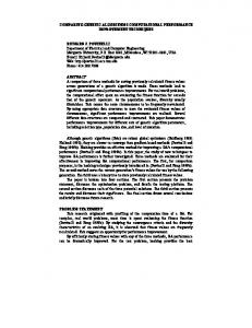
chosen for mutation, the direction of the mutation is chosen randomly with probability 2 . If the parameter is farther from the edge of the range than the maximum mutation size in the direction of the mutation, then the mutated parameter is chosen using a uniform distribution over the interval between the parameter and the parameter plus or minus the maximum mutation size. If the parameter is closer to the edge of the range than the maximum mutation size, then the new value of the parameter is chosen using a uniform distribution over the interval between the parameter and the edge of the range. To make this explicit, suppose that the original parameter value is x, the range is [a, b], the maximum mutation size is M, and that the mutation has been chosen to be in the positive direction. Then the mutated parameter is chosen from the range [x, min(M,b)] using a uniform probability distribution. Experiments indicated that this mutation scheme, when applied repeatedly to a point in an interval without selection pressure, gave an almost uniform distribution of points over a large number of mutations. The above mutation method does not correspond very closely to the mutation in a binary coded algorithm, in that the binary-coded mutation more heavily favors mutations with a small magnitude. This is especially true if a large number of bits are used to encode each real parameter. A problem with real crossover is illustrated in Figure 2. The ellipses in the figure represent contour lines of the objective function. A local minimum is at the center of the inner ellipse. Points 1 and 2 are both relatively good points in that their function value is not too much above the local minimum. However, any point generated using crossover from these points will be much worse than either point.

-7To get around this situation, we propose another form of reproduction operator that we call linear crossover. From 3 1 1 p - p , and - 2 2 1 2 2 1 1 3 1 1 3 p + p is the midpoint of p and p , while 2 p - 2 p and - 2 p + 2 p 2 1 2 2 1 2 1 2 1 2

1

p + 1

3 p . 2 2

2

The point

lie on the line determined by p

1

1

three new points are generated, namely 2 p + 2 p , 1 2

the two parent points p and p

and p . In this paper, the best two of the three points are selected.

1

2

Linear crossover has the disadvantage that it would be highly disruptive of schemata and is not compatible with the version of the schema theorem given below.

point 1

point from crossover

point 2

Figure 2 8 Schemata Analysis for Real-Allele Genetic Algorithms As explained in Section 6, we feel that, in a binary-coded genetic algorithm for a real-parameter problem, the most meaningful schemata for functions without periodicities of power 2 are those that restrict some parameters to a subinterval of their possible range. Thus, the logical way to define a schema for a real-allele genetic algorithm is to restrict some or all of the parameters to subintervals of their possible ranges. We have already assumed that the range of parameter x is a ≤ x ≤ b . ι

i

i

i

m

Thus, parameter space is p =

∏ [a , b ] , i

and a schema s is specified by choosing real values α

i

i

i=1

and β

i

m

such that a • α • β • b . Then the corresponding subset of parameter space is i i i i symbol s to refer either to the sequence of pairs ((α , β ), . . . , (α 1

1

m

,β

m

))

∏ [a , b ] . i

i

We will use the

i=1

or the corresponding subset of

m

parameter space

∏ [a , b ] . i

i

i=1

We can do the same kind of analysis that is done for traditional genetic algorithms. For this analysis, the important thing about a schema is which parameters it restricts. To each schema s we associate a template as follows. If a parameter is unrestricted, i. e., α = a and β = b , then we associate a * with that parameter. If a parameter is i

i

i

i

restricted, i. e. α > a or β < b , then let I denote its interval [a ,b ]. Then the template is the sequence of I i i i i i i i i 's and *'s corresponding to the parameters. For example, if parameter space is [-1,1] × [-1,1] × [-1,1], and if the schema is [-1,1] × [0,1] × [-1,0], then the corresponding m-tuple would be *I I . 2 3

-8Let the average fitness of the population members which are in schema s be f(s), and let the average fitness of all population members be f . Suppose that we use one-point crossover with a randomly selected crossover point. If selection and sampling are done so that the probability of an individual being selected for reproduction is the ratio of its fitness to the average fitness of the population, then the expected proportion of individuals of schema s that are selected for reproduction is:

p(s, t + 1) ≥ p(s, t)

d(s) f(s)   (1 − p(s, t)) (1 − M) F 1 − C  l −1 f 

In this equation, 1 is the chromosome length, F is the number of restricted (fixed) genes, δ(s) is the defining length (the distance between its outermost restricted genes), C is the probability of crossover, and M is the probability that a gene will be mutated. The above is Holland’s Schema Theorem (Corollary 6.4.1 of [Holland, 1975]), and is stated for genetic algorithms with any discrete set of alleles for each gene. The proof of the Schema theorem depends neither on the form of the objective function nor on how the restricted genes are restricted. Thus, it also applies to real-coded genetic algorithms using real mutation and real crossover as reproduction operators. (In the real case, the chromosome length 1 is the number of real parameters m.)

9 Experimental Results The above algorithm was implemented by modifying the Genesis program of John Grefenstette. The five problems of De Jong (F1 to F5) [De Jong, 1975] plus problems F6 and F7 of [Schaffer, Caruana, Eshelman, and Das, 1989] were included, along with two additional problems. Problem F5R is De Jong’s problem 5 (Shekel’s Foxholes) rotated 30 degrees in the plane before evaluating. Thus, the formula for F5R is: 3

1

1

3

f (x ,x ) = f ( 2 x +2x ,-2x + 2 x ) 1 2 1 2 5r 1 2 5 where f

5

is De Jong’s f5 (Shekel’s Foxholes). The last function, F8, corresponds to the solution of the following

system of 5 equations in 5 unknowns: 2

xk +

5

∑xi - 4 = 0

for k = 1, 2, . . . , 5.

i=1

This system was converted to the objective function for an optimization problem by summing the absolute values of the left sides of the above equations. The parameter ranges for all variables was −7 ≤ x k ≤ 0 . In this region, there is a single multiplicity 1 solution (global minimum): (-4, -4, -4, -4, -4). There are a number of local minima on the edges of the region. The global minimum for all problems had an objective function value of zero. All problems were run with two point crossover, the elitist strategy, Baker’s selection procedure, a scaling window of 5 generations, a population size of 20, and a crossover rate of 0.8. For the binary-coded algorithm, Gray coding was used. Both spinning and convergence thresholds were turned off. For all functions except F8, each experiment consisted of running the genetic algorithm for 1000 trials (function evaluations). For function F8, 5000 trials were used. Two results were saved for each experiment: the best performance, and the offline performance. The best performance is the smallest value of the objective function obtained over all function evaluations. The offline performance is the average over function evaluations of the best value obtained up to that function evaluation. In order to select good parameter settings, multiple runs were done for both the binary and the real-coded algorithms with different settings for mutation rates (real and binary) and mutation sizes (real). What is presented below are the best results over all of these settings of the mutation parameters. For the binary-coded algorithm, 1000 experiments were done at each mutation rate from 0.005 to 0.05 in steps of 0.005. Thus, for each function, 10 mutation rates were tried. For the real-coded algorithm using real crossover only,

-91000 experiments were done at each combination of a mutation size and a mutation rate. The mutation sizes ranged from from 0.1 to 0.3 in steps of 0.1, and mutation rates ranged from 0.05 to 0.3 in steps of 0.05. Thus, for each function, 18 combinations of mutation size and rate were tried. The same was done using 50% real crossover and 50% linear crossover. For each function and each type of algorithm (binary, real with all real crossover, and real with both real and linear crossover), the mutation settings that gave the optimal performance measure is shown below. The standard deviation is computed over the 1000 experiments at that mutation setting.

Table 1: Best Values of Best Performance Type of Algorithm

Function

Mutation Rate

Mutation Best Size Performance

Standard Deviation

Binary Real Real/linear

F1 F1 F1

0.035 0.300 0.050

0.2 0.1

0.0062 0.00058 0.00004

0.0111 0.00102 0.00004


F2 F2 F2

0.050 0.300 0.300

0.3 0.1

0.0192 0.0119 0.0107

0.0326 0.0237 0.0200


F3 F3 F3

0.030 0.300 0.300

0.3 0.3

1.4740 1.0490 0.5730

0.9012 1.0908 0.9506


F4 F4 F4

0.015 0.300 0.200

0.2 0.1

9.7311 3.5671 -1.0906

4.0645 1.9498 0.7828


F5 F5 F5

0.050 0.300 0.1

0.3 0.2

1.0116 10.5626 9.7598

0.1795 7.5863 6.5275


F5R F5R F5R

0.045 0.200 0.150

0.3 0.2

8.6699 11.7435 11.4997

5.7736 6.5181 6.2822


F6 F6 F6

0.050 0.100 0.050

0.3 0.1

0.0310 0.2071 0.0200

0.0414 0.1261 0.0266


F7 F7 F7

0.050 0.250 0.050

0.3 0.1

0.5888 2.9721 0.0584

0.3751 1.3622 0.0256


F8 F8 F8

0.040 0.150 0.050

0.3 0.3

0.36223 0.8290 0.1783

0.9677 3.5439 1.5616

- 10 -

Table 2: Best Values of Offline Performance Type of Algorithm

Function

Mutation Rate

Mutation Offline Size Performance

Standard Deviation


F1 F1 F1

0.045 0.300 0.050

0.3 0.2

0.5094 0.4871 0.3604

0.2553 0.2831 0.1483


F2 F2 F2

0.030 0.300 0.150

0.1 0.1

1.2453 1.2018 1.1673

1.0705 1.0537 1.0104


F3 F3 F3

0.030 0.300 0.50

0.3 0.3

4.4235 4.2511 3.6280

0.9691 1.3463 1.2226


F4 F4 F4

0.015 0.300 0.050

0.2 0.1

36.3860 32.0367 6.8157

7.6296 6.9149 1.9028


F5 F5 F5

0.045 0.300 0.300

0.3 0.3

14.1197 34.1292 23.3482

12.1777 38.5147 14.2119


F5R F5R F5R

0.045 0.200 0.250

0.3 0.3

19.9376 34.8737 24.3253

9.5545 30.3235 14.8582


F6 F6 F6

0.050 0.100 0.050

0.3 0.1

0.1087 0.2231 0.0757

0.0625 0.1197 0.0354


F7 F7 F7

0.050 0.250 0.050

0.3 0.2

1.7961 3.2571 1.0746

0.6009 1.2362 0.2234


F8 F8 F8

0.040 0.150 0.050

0.3 0.1

3.4175 3.0374 1.9604

1.8448 3.5018 1.6075

9.1 Summary of Experimental Results The real-coded algorithm with 50% real crossover and 50% linear crossover was better than the real-coded algorithm with 100% real crossover on all problems. (However, the differences for both best and offline performance for F2, and for best performance for F5R are of questionable significance.) The real-coded algorithm with both types of crossover was better than the binary coded algorithm on 7 of the 9 problems, and the real-code algorithm with real crossover was better than the binary-coded algorithm on 5 of the 9 problems. On problems F4 and F7 the mixed crossover real-coded algorthm did much better than the other two algorithms. On Problem F5, the Shekel’s Foxholes problem, the binary coded algorithm did much better than the real-coded algorithms This problem has periodicities that make it well-suited to a binary-coded algorithm. When the problem was rotated by 30 degrees to get rid of some of these periodicities as function F5R, the real-coded algorithms did better than before, but still not quite as well as the binary coded algorithm.

- 11 -

10 Conclusions Crossover and mutation in binary-coded genetic algorithms were analyzed as they apply to real-parameter optimization problems. This analysis suggested that binary crossover can be viewed as real crossover plus a perturbation. Real-coded genetic algorithms with two types of crossover were presented. The above analysis implies that mutation rates for real-coded algorithm should be considerably higher than for binary-code algorithms. For one of these types of crossover (real crossover), Holland’s Schema Theorem applies easily. Experimental results showed that the real-coded genetic algorithm based on a mixture of real and linear crossover gave superior results to binary-coded genetic algorithm on most of the test problems. The real-coded algorithm that used linear crossover in addition to real crossover outperformed the real-coded algorithm that used all real crossover on all test problems. The strengths of real-coded genetic algorithms include: (1) Increased efficiency: bit strings do not need to be converted to real numbers for every function evaluation. (2) Increased precision: since a real-number representation is used, there is no loss of precision due to the binary representation. (See also [Schraudolph, 1991] in these proceedings.) (3) Greater freedom to use different mutation and crossover techniques based on the real representation. The work of Schwefel, Rechenberg, and other proponents of Evolutionsstrategie is relevant here. However, the greater freedom mentioned in (3) can give practitioner more decisions to make and more parameters to set. Acknowledgements The author would like to thank his student Kevin Lohn for conversations, and Digital Equipment Corporation for the loan of a DECStation 3100 on which some computer runs were done. References Antonisse, Jim, (1989) A new interpretation of schema notation that overturns the binary encoding constraint. In J. David Schaffer, (ed.), Proceedings of the Third International Conference on Genetic Algorithms, San Mateo, CA: Morgan Kaufman Publishers, Inc., 86-91. Davis, Lawrence, (1989) Adapting operator probabilities in genetic algorithms. In J. David Schaffer, (ed.), Proceedings of the Third International Conference on Genetic Algorithms, San Mateo, CA: Morgan Kaufman Publishers, Inc., 61-69. De Jong, K. A., (1975) Analysis of the behavior of a class of genetic adaptive systems. Ph.D. Dissertation, Department of Computer and Communications Sciences, University of Michigan, Ann Arbor, MI. Goldberg, David E. (1989). Genetic Algorithms in Search, Optimization, and Machine Learning. Massachusetts: Addison-Wesley.

Reading,

Holland, J. H. (1975). Adaptation in natural and artificial systems. Ann Arbor: The University of Michigan press. Lucasius, C. B., and G. Kateman, (1989) Applications of genetic algorithms in chemometrics. In J. David Schaffer, (ed.), Proceedings of the Third International Conference on Genetic Algorithms, San Mateo, CA: Morgan Kaufman Publishers, Inc., 170-176. Matyas, J, (1965) Random optimization. Automation and Remote Control, 26, 244-251. Price, W. L., (1978) A controlled random search procedure for global optimization. Towards Global Optimization, edited by L. C. M. Dixon and G. P. Szego, North Holland. Schaffer, J. David, Richard A. Caruana, Larry J. Eshelman, and Rajarshi Das, (1989) A study of control parameters affecting online performance of genetic algorithms for function optimization. In J. David Schaffer, (ed.), Proceedings of the Third International Conference on Genetic Algorithms, San Mateo, CA: Morgan Kaufman Publishers, Inc., 51-60.

- 12 Schraudolph, Nicol N., and Richard K. Belew, (1991) Dynamic Parameter Encoding for Genetic Algorithms, These proceedings. Schwefel, H., (1981) Numerical Optimization of Computer Models, (M. Finnis, Trans.), Chichester: John Wiley. (Original work published 1977).