Genetic programming as a model induction engine - CiteSeerX

35

© IWA Publishing 2000

Journal of Hydroinformatics

|

02.1

|

2000

Genetic programming as a model induction engine Vladan Babovic and Maarten Keijzer

ABSTRACT Present day instrumentation networks already provide immense quantities of data, very little of which provides any insights into the basic physical processes that are occurring in the measured medium. This is to say that the data by itself contributes little to the knowledge of such processes. Data mining and knowledge discovery aim to change this situation by providing technologies that

Vladan Babovic Maarten Keijzer Danish Hydraulic Institute, Agern Alle´ 5, DK-2970 Hørsholm, Denmark

will greatly facilitate the mining of data for knowledge. In this new setting the role of a human expert is to provide domain knowledge, interpret models suggested by the computer and devise further experiments that will provide even better data coverage. Clearly, there is an enormous amount of knowledge and understanding of physical processes that should not be just thrown away. Consequently, we strongly believe that the most appropriate way forward is to combine the best of the two approaches: theory-driven, understanding-rich with data-driven discovery process. This paper describes a particular knowledge discovery algorithm—Genetic Programming (GP). Additionally, an augmented version of GP—dimensionally aware GP—which is arguably more useful in the process of scientific discovery is described in great detail. Finally, the paper concludes with an application of dimensionally aware GP to a problem of induction of an empirical relationship describing the additional resistance to flow induced by flexible vegetation. Key words

| data mining, knowledge discovery, genetic programming

INTRODUCTION In making the most of a set of experimental data it is

constitutes a model of that object, process or event

generally desirable to express the relation between the

(Abbott 1993). Data, on the other hand, remain as ‘mere’

variables in the form of an equation. In view of the

data just to the extent that they remain a collection of signs

necessarily approximate nature of the functional relation,

that does not serve as a sign. From this point of view, the

such an equation is described as ‘empirical’. No particular

evolution of an equation within a physical symbol system

stigma should be attached to the name since many

as a means of better conveying the ‘meaning’ or ‘semantic

ultimately recognised chemical, physical and biological

content’ that is encapsulated in the data, corresponds to

laws have started out as empirical equations.

the evolution of another kind of sign and thereby consti-

Sciences devote particular attention to the develop-

tutes a model. Evidently the ‘information content’ is very

ment of a physical symbol system, such as a scheme of

little changed, or even unchanged, but the ‘meaning value’

notation in mathematics, together with the evolution of

is commonly increased immensely. Since it is just this

more refined representations of physical and conceptual

increase in ‘meaning value’ that justifies the activity of

processes in the form of equations in the corresponding

substituting equations for data, there is a natural

symbols. It is a common experience that one and the same

interest in processes for further promoting such means.

physical symbol system may serve for the expression of a

The formation of modern sciences occurred approxi-

great number of different equations. Since each equation

mately in the period between the late fifteenth century and

can be regarded as a collection of signs that serves as a sign

the late eighteenth century. The new foundations were

for a particular physical object, process or event, so it

based on the utilisation of the concept of a physical

36

Vladan Babovic and Maarten Keijzer

|

Genetic programming as a model induction engine


|

02.1

|

2000

experiment and the applications of a mathematical

data have to offer. Only a very small percentage of the

apparatus in order to describe these experiments. The

captured data is ever converted to actionable knowledge.

works of Brahe, Kepler, Newton, Leibniz, Euler and

Owing to the data – and information – overflow, the tra-

Lagrange clearly exemplify such an approach. Before

ditional approach of a human analyst, intimately familiar

these developments, scientific work primarily consisted

with a data set, serving as a conduit between raw data and

only of collecting the observables, or recording the

synthesised knowledge by producing useful analyses and

‘readings of the book of nature itself’.

reports, is breaking down.

This novel scientific approach was principally charac-

What to do with all this data? Ignoring whatever we

terised by two stages: a first one in which a set of obser-

cannot analyse would be wasteful and unwise. This is

vations of the physical system are collected, and a second

particularly pronounced in scientific endeavours, where

one in which an inductive assertion about the behaviour

data represent carefully collected observations about

of the system – a hypothesis – is generated. Observations

particular phenomena that are under study.

represent specific knowledge, whereas a hypothesis repre-

However, mining the data alone is not the entire

sents a generalisation of these data that implies and

story. At least not in scientific domains! Scientific

describes observations. One may argue that through this

theories encourage the acquisition of new data and these

process of hypothesis generation one fundamentally

data in turn lead to the generation of new theories.

economises thought, as more compact ways of describing

Traditionally, the emphasis is on a theory, which

observations are proposed.

demands that appropriate data be obtained through

Today, in the late 20th century, we are experiencing

observation or experiment. In such an approach, the

yet another change in the scientific process as just out-

discovery process is what we may refer to as theory-

lined. This latest scientific approach is one in which infor-

driven. Especially when a theory is expressed in

mation technology is employed to assist the human

mathematical form, theory-driven discovery may make

analyst in the process of hypothesis generation. This

extensive

computer-assisted analysis of large, multidimensional data

mathematics and with the subject matter of the theory

sets is sometimes referred to as a process of ‘data mining

itself. The converse view takes a body of data as its starting

use

of

strong

methods

associated

with

and knowledge discovery’ (Fayyad et al. 1996). Data

point and searches for a set of generalisations, or a theory,

mining and knowledge discovery aims at providing tools

to describe the data parsimoniously or even to explain

to facilitate the conversion of data into a number of forms

it. Usually such a theory takes the form of a precise

that convey a better understanding of the processes that

mathematical statement of the relations existing among

generated or produced these data. These new models,

the data. This is the data-driven discovery process.

combined with the already available understanding of the

Most of the applications of data mining technology are

physical processes—the theory, can result in an improved

currently in the financial sector. There is a very strong

understanding and novel formulations of physical laws

economic incentive to apply state-of-the-art technology

and an improved predictive capability.

for commercial benefits. Additionally, this domain is,

As we enter the true digital information era, one of the

relatively speaking, theory-poor, and the generation of

greatest challenges facing organisations and individuals is

new ‘black-box’ tools based solely on observations is

how to turn their rapidly expanding data stores into acces-

accepted with little scepticism. In scientific applications,

sible, and actionable, knowledge (Fayyad et al. 1996).

the situation is quite different. Clearly, there is an

Means for data collection and distribution have never

enormous amount of knowledge and understanding of

been so advanced as they are today. While advances in

physical processes that should not just be thrown away.

data storage and retrieval continue at an extraordinary

We strongly believe that the most appropriate way for-

rate, the same cannot be asserted about advances in infor-

ward is to combine the best of the two approaches: theory-

mation and knowledge extraction from data. Without such

driven, understanding-rich with data-driven discovery

developments, however, we risk missing most of what the

processes.

37


|


SYMBOLIC REGRESSION


|

02.1

|

2000

Crick, Watson and others in the 1950s, distinguishes between an organism’s genotype, which is constructed of

Regression – linear or nonlinear – plays a central role in

genetic material that is inherited from its parent or

the process of finding empirical equations. In its most

parents, and the organism’s phenotype, which is the com-

general form, regression techniques proceed by selecting a

ing to full physical presence of the organism in a certain

particular model structure and then estimating the

given environment and is represented by a body and its

accompanied coefficients based on the available data. The

associated collection of characteristics or phenotypic

model structure can be linear, polynomial, hyperbolic,

traits. Within this paradigm, there are three main criteria

logarithmic, etc. The only requirement in such an

for an evolutionary process to occur (Maynard Smith

approach is that the coefficients in the model can be

1975):

estimated using an optimisation technique. In generalised

•

linear regression for instance, the only requirement is that the model is linear in the coefficients. The model itself can consist of any functional form. Another technique may be a nonlinear regression where the only requirement is that

•

the model is differentiable both in the inputs and the coefficients. Supervised artificial neural networks belong to this class of regression techniques. In this paper a relatively novel regression technique, symbolic regression (Koza 1992) is described. The specific model structure is not chosen in advance, but is part of the

•

Criterion of Heredity:

Offspring are similar to

their parents: the genotype copying process maintains a high fidelity. Criterion of Variability:

Offspring are not exactly

the same as their parents: the genotype copying process is not perfect. Criterion of Fecundity:

Variants leave different

numbers of offspring: specific variations have an effect on behaviour and behaviour has an effect on reproductive success.

search process. In this algorithm, both model structure

It can be shown that these three requirements provide

and coefficients are simultaneously being searched for.

necessary and sufficient conditions for an evolutionary

The user has to define some basic building blocks

process to occur, so that they define the grammar of the

(function and variables to be used); the algorithm tries to

corresponding ‘language’, whether this be written in

build a model using only those specified blocks. As the

strings of nucleotides, or amino acid molecules, or in

space of model structures is in general not smooth, not

strings of binary digits, or in strings of symbols, or what-

differentiable nor linear in any useful sense (it is in fact

ever. The criterion of heredity ensures that the offspring

highly discontinuous), standard optimisation techniques

inherits information from its parents, assuring similarity.

fail when trying to find both the model structure and the

Variability is guaranteed in any entropy-producing system,

coefficients.

whereas the criterion of fecundity provides, on average,

The only information available for the symbolic

more fit individuals with the possibility to reproduce

regression problem is the error that a particular model

more often and thus generate more and better-surviving

makes. No auxiliary information about gradients is avail-

offspring.

able. The class of evolutionary algorithms, therefore,

The application of these evolutionary principles

seems to be one of the few methods able to perform an

results in an adaptation of a population to an environ-

effective search in this domain.

ment. Adaptation can in turn be conceived as a process of accumulation of knowledge (see, for example, Margalef 1968). Since Darwinism is a theory of processes of cumu-

The evolutionary paradigm The paradigm of evolutionary processes, as established

lative adaptation, it can best be conceived within the present perspective as a theory of accumulation of knowledge about an environment.

by Darwin and Weismann in the 19th century, and pro-

The first proposal to apply the creative power of the

vided with its information-theoretic interpretation by

evolutionary process in more general terms than the

38


Table 1

|

|


Pseudo-code for evolutionary algorithm.


|

02.1

|

2000

The structures undergoing adaptation Owing to the many different types of evolutionary algorithm defined, it is difficult to develop a formal framework for describing evolving genotypes. For linear genotypes such as those used in most genetic algorithms and evolution strategies, Radcliffe & Surry (1994) showed that an individual’s genotype v can be coded as a string of l genes. Each of these genes can take on values from some (typically, but theoretically necessarily not finite) set Ai. Accordingly, the genotypic representation space V takes the form: V = A1 × A2 × A3 . . . × Al .

(1)

In classical Genetic Algorithms (GAs), as introduced by biological can be traced back at least as far as the work

Holland (1975), the elements aki of the sets Ai typically

of Cannon (1932: see Harvey 1993). The first working

take on binary values:

computer algorithm that realised this approach – that of Evolutionary Operation (EVOP) – is attributed to Box

∀ aki ∈ Ai,

aki ∈ {0,1} .

(2)

(1957). Works of Friedberg (1958) and Bremermann (1958) provided some inspiring results but were not well accepted

In Evolution Strategies (ES), on the other hand, the

by the contemporary scientific community (e.g. Minsky

elements aki are real-valued numbers, i.e.

1963). In time, however, research in evolutionary algorithms

∀ aki ∈ Ai,

aki ∈ R .

(3)

overcame most of the problems that both Friedberg and Bremermann had encountered. More than three decades

In these cases we can regard the set of distinct elements aki

of research have resulted in differentiation into four main

as an alphabet. In Evolutionary Programming (EP) the

streams of Evolutionary Algorithm (EA) development:

sets Ai are more broadly defined and can be adapted to any

namely those of Evolution Strategies (ES) (Schwefel 1981);

problem at hand, ranging from numerical optimisation

Evolutionary Programming (EP) (Fogel et al. 1966);

(Fogel 1992), through finite-state automation evolution

Genetic Algorithms (GA) (Holland 1975); and Genetic

(Fogel 1993) to connectionist network induction (Fogel

Programming (GP) (Koza 1992). However, all evolutionary

et al. 1990).

algorithms share the common property of applying evol-

The phenotype x of an evolving entity is an interpret-

utionary processes in the form of selection, mutation

ation of a genotype v in a problem domain. In the case of

and reproduction on a population of individual structures

GAs, a typical genotype v composed of l ‘letters’ or ‘words’

that undergo evolution. The general process is illustrated

may appear in a more general form as v (a1 × . . . × a1) ∈V.

in the form of a pseudo-code in Table 1. The criterion of

For example, when a particular ai takes values of 0 or 1, then

heredity is assured through the application of a crossover

the genotype simply takes the form of a binary string, such

operator, whereas the criterion of variability is maintained

as:

through the application of a mutation operator. A selection mechanism then ‘favours’ the more fit entities so that

v = 1 0 0 1 1 0 1 1.

(4)

they reproduce more often, providing the fecundity requirement necessary for an evolutionary process to

To extract any useful meaning, this code has to be

proceed.

interpreted in some way, and indeed in this case the

39


|



|

02.1

|

2000

interpretation is the individual’s phenotype x. The mapping

is its rudimentary alphabet, consisting only of 0s and

between genotypes and phenotypes then depends only on

1s or other such sign pairs. Moreover, in the case of a GA

the admitted physical symbol system—and the developers’

there is in principle nothing preventing the application

ingenuity. For example, if a binary string is to be interpreted

of a mapping in which, for example, 100 would stand

as a phenotype that is characterised by two traits that have

for x1, 11 for + and 011 for x2, so that the binary

numerical measures x1 and x2 only, defined on domains [xˇ1,

representation of the genotype as exemplified in Equation

xˆ1] and [xˇ2, xˆ2] respectively, a simple mapping can always be

(4) above would become a phenotype with an interpret-

found that will provide this interpretation. For example, in

ation (x1 + x2).

the case of Equation (4), where l = 8, we can subdivide the

Clearly, phenotypes generated applying this last

genotype into, say, two equinumerous intervals of length

mapping and a mapping of the kind exemplified in

Lx = l/2 = 4, and apply the following general mapping:

Equation (5) are meant for different purposes. The latter are typically used for optimisation and constraint satisfaction applications. For a general overview see Goldberg (1989) and, for applications in a water-related domain, Babovic (1993, 1996).

where aj is the value of the numeral in the binary string and

A third route of genotype to phenotype mapping is

b is the base number. In this way a genotype v is interpreted

present in genetic programming (GP) (Koza 1992). Instead

as a phenotype x with just two traits, in this case of the form

of using the identity mapping as in evolution strategies or

x1 [0, 10] and x2 [0, 10], according to the scheme exempli-

keeping it completely open such as in genetic algorithms,

fied in Equation (5) as follows:

genetic programming restricts the mapping from genotype to phenotype such that the phenotype is executable in the same sense as a computer program is executable. Problems tackled by genetic programming are then problems of program induction. Although this limits the scope of genetic programming, it remains broad enough to encompass seemingly remote problems such as: model induction, symbolic regression, optimal control, planning, sequence induction, discovering game-playing strategies, empirical discovery and forecasting, symbolic integration and differentiation, inverse problems and induction of decision trees. In his monograph, Koza (1992) argues (chapter 2, p. 9):

Thus the genotype of Equation (4) generates a phenotype with two traits (6.0, 8.67), each of which is characterised by one real number. Evolution Strategies (ES), on the other hand, represent evolving entities using real-valued numbers and not binary strings. In this way the mapping between genotype and phenotype is avoided. This provides certain advantages and accelerates the algorithms, but it naturally restricts the field of application to numerical domains only. One of the main advantages of the GA

A wide variety of terms are used in various fields to describe this basic idea of program induction. Depending on the terminology of the particular field involved, the computer program may be called a formula, a plan, a control strategy, a computational procedure, a model, a decision tree, a game-playing strategy, a robotic action plan, a transfer function, a mathematical expression, a sequence of operations, or perhaps merely a composition of functions. Similarly, the inputs to the computer program may be called sensor values, state variables, independent variables, attributes, information to be processed, input signals, input values, known variables, or perhaps merely arguments to a function. The output from the computer program may be called a dependent variable, a control variable, a category, a decision,

40


|



|

02.1

|

2000

an action, a move, an effector, a result, an output signal, an output value, a class, an unknown variable, or perhaps merely the value returned by a function. Regardless of the differences in terminology, the problem of discovering a computer program that produces some desired output when presented with particular inputs is the problem of program induction.

The alphabet used in the GP code comprises a physical symbol system, so that it consists of symbolic operators, the choice of which depends only on the nature of the problem to be solved. One may, for example, choose an alphabet consisting solely of logical operators, such as AND, OR, NOT

and

IF THEN ELSE

and evolve rule-based-like

structures. One may restrict the alphabet to arithmetic– algebraic operators such as + , − , *, /, etc. so as to evolve arithmetic–algebraic formulae. On the other side of the

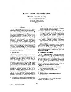
Figure 1

|

A parse tree representing the expression (p+v)*z.

symbolic spectrum, the alphabet can be chosen from operators containing side effects, memory addressing and which, together with

subsequently the search-space for genetic programming,

arithmetic and logical functions, embodies a complete

will consist of all possible mathematical expressions,

computer language.

regardless of their shape and size.

loops such as

READ, WRITE, WHILE

As computer programs (and less generally mathemati-

The great advantage of this change in representation

cal formulae) have a well defined grammar and are of

will become clear when we represent these structures in

variable size and shape, in genetic programming the struc-

tree form rather than bracketed strings. The distinction

tures undergoing adaptation are often taken from the class

between the terminals and functions (non-terminals) will

of parse trees. Parse trees are general constructs in com-

then become clear. Terminals are represented by the ex-

puter science and are used, among other things, as inter-

tremities or ‘leaves’ of the tree, like p, v or z. In addition to

mediate structures in compiling computer languages such

these, terminals may be constants that are inserted in the

as C( + + ), Pascal and Fortran. A parse tree is inductively

formulae. Functions are elements of a tree that act upon

defined in Table 2: In this definition the subscripts 0, 1,

terminals and in Figure 1 these are exemplified by + and *.

. . . , n of the sets F in L denote the arity of the functions i.e.

It follows straightforwardly from the definition in

the number of arguments they need. The set of functions of

Table 2 that replacing a child node of a well-defined

arity zero is often called the terminal set or T. When we

parse tree by an arbitrary well-defined parse tree yields a

restrict the function and terminal sets to mathematical

well-defined parse tree. It follows that:

operations, the parse trees that can be generated, and

1.

Every grammatically correct equation (and, in general, every well-formed formula, or wff) can be represented as a parse tree.

Table 2

|

Definition of parse tree.

2.

Every planar graph with grammatically correct terminals and functions represents a grammatically correct equation (or, generally, a wff).

3.

Depth and size of a wff are easily defined as the longest non-backtracking path from a leaf to the root of the tree, and the number of nodes in the tree, respectively.

41


|


When applying genetic programming using mathematical


Table 3

|

z

Koza termed symbolic regression. Symbolic regression, in functional form as well as the coefficients of a formula. Just like linear regression it works on a spreadsheet of

the form of the model does not need to be specified

|

2000

v

P

E

1

7.945

3.91

14121.67

10.94294

2

18.585

5.287

14506.06

22.91308

data, and tries to fit a model to this data. There are two unique features in symbolic regression on data. First,

02.1

Dataset for the induction of Bernoulli’s law.

functions and variables only, we have entered the field contrast with (non-)linear regression tries to find both the

|

1000

...

...

...

...

15.884

12.7

10770.01

33.42325

beforehand. A specification of the more elementary building blocks (the language L above) will do. Second, the optimisation criterion is not restricted to a class of, for example, squared error measures. As will be shown below, the optimisation does not even need to be restricted to a

Formula (6) is a simplified formulation that ignores

single objective: a multi-objective optimisation is quite

energy losses due to friction and local losses induced by

straightforward to implement.

sudden changes in a cross-section of the conduit. In

The equations so represented may be grammatically

accordance with tradition in hydraulics, energy in formu-

correct, but they may not necessarily be logically correct,

lation (6) is expressed in implicit potential energy

or ‘logical’, and then in the special but immediate sense

terms, as metres of a water column, rather than in more

that they may not necessarily be dimensionally consistent.

conventional energy units. For the purpose of induction of Bernoulli’s law a

Symbolic regression on Bernoulli’s law

specific genetic programming system will be developed in this text. This system differs in almost all aspects from a

In the remainder of this section an introduction to genetic

more ‘standard’ implementation of a genetic programming

programming specifically used in symbolic regression

system. In particular, it is almost entirely different from the

will be offered. For pedagogic purposes, an artificial

system as described by Koza (1992). There is a great degree

dataset with a known solution is chosen as a running

of freedom in implementing genetic programming systems

example. The target is to find Bernoulli’s law of energy

and there are no known optimal choices for the various

conservation:

details of the system. However, the overall design of a genetic programming system needs to address a number of issues and these are condensed in this paper.

or in a regression context, to find: The data and the terminal set First a dataset is created on the basis of the desired E = z + p/g + v2/2g

in

numeric

form

using

where:

relation

z denotes distance above a certain energy datum,

reasonable numeric values. See Table 3 for an example.

p denotes pressure,

In real-world problems a similar dataset would be all

v denotes velocity,

that is available. The object of the search is now a formula

g denotes the Earth’s gravitational acceleration

that takes z, v, and p as input and produces E as output.

2

[g = 9.81 m /s], and g denotes the specific gravity of a fluid [for water 3

g = 9810 N/m ].

The constants g and g may also be included, but in the present example only randomly generated constants will be used.

42


|



|

02.1

|

2000

The function set: sufficiency and closure The next step is to define a function set for the problem. A function and terminal set are called sufficient if they are able to represent a solution to the problem. As in this case the optimal solution is known, the optimal function set can be determined easily. In the general case, when all that

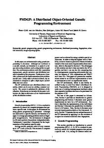
Figure 2

|

Example of the systematic specialisation of an expression.

is known is the raw data, an informed guess must be made as to what functions and terminals to use for genetic programming. For this problem we choose: Function Set { + , *, − , /, power, sin, ln}

purposeful action, in that a randomly created collection of entities can provide a satisfactory initial coverage of the search space. At the same time, computationally

There is one point that needs to be explicitly taken care of.

speaking, this is an inexpensive process that calls for no

As the crossover mechanism (as defined below) can swap

initial or preconceived knowledge from the side of the

any sub-tree to any location in the tree, it needs to be

problem-solver.

ensured that all values have the same type, and that all

The process of random initialisation of a parse tree is

functions can accept all possible inputs from terminals and

depicted in Figure 2. First, a function is randomly selected

functions and will return a well-defined value. This property

from a function set, e.g. *. This function has an arity of

is called closure. In the function set above there are three

2 and thus requires two arguments. In the next step,

functions that might violate this closure property. The div-

arguments are randomly selected from the function sets.

ision function is undefined when its second argument is

Figure 2a,b illustrates the situation in which the left

zero, the power function is undefined when a negative value

branch of a tree is fed with a function + and the right with

is raised to a non-integer power, and the natural logarithm

a terminal z. Since the left branch is non-terminal the

is undefined for values smaller and equal to zero. Other

process is repeated recursively until all the leaves of the

potential pitfalls are underflows and overflows in the

tree are terminals. This is illustrated in Figure 2c, where

floating-point implementation of these functions.

the randomly selected terminals for + are p and v.

One possible approach to satisfying closure is to

This process is repeated for every individual in a GP

protect the operators so that they return well-defined

population of size N. It should be noted that such a

values when confronted with illegal inputs (Koza 1992). A

creation of parse trees results in the generation of geno-

protection for division might be to return the value 1 when

types of variable length. To restrict the size of the initial

confronted with a division by zero. For the power function

population, a maximum depth parameter D may often be

a solution could be to use complex numbers instead.

supplied. Several different initialisation procedures exist

Similarly, one can also define protections for the square

for GP; some of them are described below.

root and logarithm functions. Another approach (which is adopted here) is to use a special undefined value NaN that

Full method

is returned by functions with illegal inputs. All functions

Assign zero probability to the terminal set T and uniform

that receive NaN in any of their inputs will also return NaN. Finally, the objective function will return the worst possible value when one of the inputs is NaN.

probability to the remaining functions from L. Generate a tree consisting of non-terminals only until the depth D is reached. Then assign uniform probability to the members of T and zero to the remaining functions from L, thus completing the tree with terminals.

Initialisation of genetic programming Evolutionary algorithms are typically initialised by

Grow method

creating an initial population randomly. This is in fact a

Assign uniform probability to all functions from L. If the

43


|


depth of the tree reaches D generate terminals only. This


Table 4

|

|

02.1

|

2000

Pseudo-code for initialization on size.

will result in variable shaped and sized trees.

Ramped half-and-half A combination of the full and grow methods. Generate for each of the depths from 2 to D an equal number of trees using grow and full methods in equal proportions. This method is preferred by Koza (1992) as it generates parse trees of various shapes and sizes and consequently provides a good coverage of the search space. This initialisation procedure is less sensitive to the ratio of functions over terminals than the grow method by itself.

Exact uniform initialisation

algorithm it is only necessary to include the terminal set in

None of the methods above succeeds in generating parse

the sets of functions in line 4 (marked with *) of the

trees distributed uniformly over the space of all possible

pseudo-code above. This implementation method gives

parse trees up to depth D. As there are exponentially more

better control of the size of the initial parse trees.

parse trees of depth D than of depth D − 1, the ramped

In our running example of induction of Bernoulli’s

half-and-half method is biased towards generating trees of

law, a variant of the grow initialisation on size is employed

smaller depths. (The exact relation between the number of

with S = 15, N = 4 and D = 4, and provides, for example,

possible parse trees over increasing depth is given by

the following kinds of expressions:

Lz D i D n(D + 1) = ∑z i=1 zF iz∑ j=1n(j) − ∑ j=2n(j), where n(D) is

the number of parse trees at a certain depth and n(1) is the size of the terminal set F0 or T. The recursion can be verified by considering that a tree of depth D + 1 has children that are maximally D deep, given by the first summation. As the first summation calculates the number

When a constant is created its value is set to the ratio of

of parse trees up to depth D + 1 including all trees from

two independent uniform random variables.

depth 2 to D, subtracting the second summation will give the exact result of all trees of a specific depth.) Bohm & Geyer-Schultz (1996) suggest using the recursion above to

Objective functions, selection and fitness

generate trees uniformly over all depths and shapes, such

Although it is often claimed that evolutionary algorithms

that every parse tree up to depth D has an equal

embody a computer-based version of natural selection

probability of being generated.

(Koza 1992), this is not the case when they are used in an optimisation context. In contrast with optimisation,

Initialisation on size

evolution is not goal-oriented in an optimisation sense. The only goal orientation that might be distinguished is

Instead of using a maximum initial depth parameter D,

that organisms are optimised in their ability to create

use an initial size parameter S, and initialise using the

offspring. All traits in all their wonderful complexity are

pseudo-code from Table 4.

mere side-effects of this all-encompassing goal.

This implements a full method on size, as every tree will be of exact size S. To create a grow variant of this

To

continue

drawing

analogies

with

biology,

evolutionary algorithms as used for optimisation purposes

44


|



|

02.1

|

2000

are more akin to breeding. If one wants to optimise some

Selection is the optimisation force within the

trait in, for example, pea plants, one will proceed by

evolutionary algorithm, keeping it focused on the

breeding with those plants that exhibit most of the specific

worthwhile regions of the search-space by mapping

trait to breed. These plants will be crossbred and grown

the objective function values to the number of offspring

again. By applying this procedure for a number of gener-

produced. Selection generally reduces the population to

ations, the average quality of a trait of interest in the

its observed best members; the population is subsequently

pea plants will increase. Contemporary agriculture is

enlarged by the mutation and crossover operations on the

extensively optimised using this technique.

selected members. Several selection mechanisms have

Evolutionary algorithms in optimisation proceed in a similar fashion. First an objective function is defined that usually takes the form of a scalar value that is applied to every population member: o:Fx→R

been proposed for evolutionary algorithms. Three of the most popular mechanisms are described here. 1.

Truncation Selection simply keeps the best proportion of t of the population and discards the rest. The parameter t then governs the selection

(8)

mapping the outputs of the formula Fx to a real-valued scalar. When using genetic programming to find equations

intensity of the mechanism. Evolution strategies (Schwefel 1981) use only this mechanism. 2.

that approximate data (i.e. symbolic regression), the objec-

selects the best as the winner. In a steady-state

tive functions used are often error measures of some form.

algorithm a subsequent tournament is held for

This measure can simply be a root mean squared error, but

finding a partner and an inverse

also the number of points correctly predicted within some

tournament – selecting the worst individual – can be

accuracy interval of tolerance (the number of correctly

held to find a slot to fit in one of the offspring. The

predicted data points is often called the number of hits of

tournament size parameter k governs the selection

the population member). Since a population member within a genetic programming computes some function f using the input vectors x, the error in producing the desired outputs y can be computed with any cost or error function. To compare objective function values, it is often enough to supply information a to whether this function should be minimised or maximised. Again, it is not necessary that the objective function is continuous nor is it necessary for it to be differentiable, as an evolutionary algorithm does not use this information. The objective function chosen in the running example

k-Tournament Selection proceeds by holding tournaments of k randomly selected individuals and

intensity here. 3.

Fitness Proportional Selection assigns every individual in the population a probability proportional to its objective function value. Selection is then governed by these probabilities. To obtain these probabilities the objective function needs first to be scaled to a non-negative quantity. This transformation from raw objective scores to a non-negative quantity is called the fitness function (Grefenstette 1997).

of Bernoulli’s law induction is the root mean squared error

Although fitness proportional selection is one of the most

(RMS), given by:

frequently used selection mechanisms in genetic algorithms (and in fact the schema theorem (Holland 1975) depends on it), it is also one of the most cumbersome to use. The objective function values need to be transformed

After calculating the objective function values for all

and scaled. To vary the selection intensity, several scaling

population members, the following step is to create the

mechanisms have been devised, often utilising some prop-

next generation. Similarly, as in breeding, the better

erties of the particular objective function used. In effect,

solutions will have a larger expected number of offspring.

such scaling mechanisms implement the entire selection

This step is referred to as selection.

mechanism, as fitness proportional selection by its very

45


|



|

02.1

|

2000

nature is a method that ‘merely’ translates values into

so-called Pareto ranking, where the concept of dominance

probabilities. Likewise all other selection mechanisms

plays an important role. When working with more than

can be translated as scaling mechanisms for fitness pro-

one objective, a solution is said to be dominant over

portional selection through a straightforward, although

another solution of the problem when it is better on at

tedious, calculation of probabilities. (A cautionary remark

least one objective and not worse on any of the others. The

should be issued that owing to the relatively small sizes of

Pareto ranking method assigns each population member a

evolutionary algorithm populations, the effect of sampling

rank based on the number of members that it dominates

error is non-negligible.)

(Foseca & Fleming 1995). In this fashion the solutions at

In his first treatise on GP, Koza (1992) used only

the front of non-dominated solutions will get the best

fitness proportional selection, and subsequently inter-

rank, zero. Goldberg (1989) proposed an alternative

mediate scaling methods such as standardised, adjusted

Pareto ranking method. The first non-dominated solutions

and finally normalised ‘fitness’. The subsequent volume

are assigned rank zero and are subseqently removed from

(Koza 1994) and most of the current implementations of

consideration. The remaining non-dominated solutions in

genetic programming use tournament selection on a

the population receive a rank of one and the process is

steady-state population. This selection mechanism has the

repeated. Both Pareto ranking methods succeed in achiev-

advantage (together with truncation selection) that the

ing the goal of multi-objective optimisation: no preference

objective function values are only compared and the map-

is given to either objective and all non-dominated

ping from objective function values to expected number of

solutions are assigned the same rank.

offspring is then implicitly (albeit with sampling error)

For the problems of symbolic regression a very natural second objective, in addition to the error measures, is the

performed by the selection mechanism. In our Bernoulli example truncation selection with a

complexity, or size, of the solution. Instead of using

truncation percentage of 15% has been chosen. This is

weighting schemes such as regularisation or minimum

applied on a population size of 500. Truncation selection

description length, Pareto ranking methods as described

has been chosen for its ease in implementation. The popu-

above serve equally well. The only disadvantage may be

lation is sorted using the RMS error, the worst 85% of the

that at the end of the run, the user is confronted with a

population are deleted, and the remaining part of the

front of solutions instead of a single solution.

population is filled with variants of those 15% survivors. This implements rather high selection intensity. In this section symbolic regression was treated using a single objective (an error measure). Evolutionary algor-

Population models

ithms are, by virtue of their population-based search, well

There are several population models in addition to the

suited for a multi-objective approach. With a number of

existence of the already described steady-state population,

objectives to optimise on, evolutionary algorithms can

where the population size remains unaltered during a run

develop

non-dominated

(or is decreased and increased by one, in another view-

solutions by employing fairly simple mechanisms of

point). Another frequent population structure is a

dominance. This is particularly useful when no a priori

so-called generational model, where an intermediate

preference or weighting scheme on the objectives is

mating pool is produced where the selected individuals

possible. The generalised objective function in multi-

reside in order to form the next generation of offspring.

objective optimisation takes the form:

The mating pool is populated by applying truncation,

the

entire

Pareto-front

of

tournament or fitness-proportional selection. Whether o:Fx→Rn,

(10)

some members of the mating pool are simply copied (reproduced) to the next generation or not defines

where n is the number of objectives. One way of imple-

whether the population model is elitist or not. Elitism

menting a multi-objective mechanism is by a means of a

ensures that the best population member(s) survive the

46


|



|

02.1

|

2000

generation gap in order to keep the best-so-far solution(s)

resulting offspring are grammatically (and, specifically,

in the evolving population. Tournament selection within a

syntactically) correct. The first efforts of the GA com-

steady-state model is naturally elitist in that the best

munity to evolve symbolic expressions (Cramer 1985) were

member is maintained in the population when the inverse

based on the interpretation of a binary string in symbolic

tournament is held through picking members without

form. Despite some limited successes of this approach, it

replacement.

was found that it still necessitated an extensive checking

Another distinction in population structure can be

of the grammatical correctness of the resulting formulae,

made through panmictic and distributed populations. A

and in cases when the resulting expressions were not

panmictic population is thoroughly mixed. Selection oper-

correct it necessitated patching and other methods of

ates on a global scale, taking the fitnesses of the entire

rehabilitation. In certain cases, the algorithm was

population into account. A distributed population is dis-

even found to spend most of its time carrying out these

tributed in a certain spatial sense, and selection operates

rehabilitation measures.

locally. Examples of such distributed population models

In view of these difficulties, Koza (1992) followed a

are: the island model in which there are independently

somewhat different path, in which parse trees were

evolving sub-populations, with the occasional migration

manipulated directly in an evolutionary process. The

of individuals between islands to exchange genetic

consequence of this approach is that the syntax of the

material; and the diffusion model where the population is

formulae

distributed within a one-, two- or multi-dimensional grid

regardless of the crossover site. There is then no need for

in which local mixing and selection occur. By distributing

additional corrections and patching. As remarked earlier,

the population some parallel evolution can occur, making

this means that the grammatical correctness of statements

the algorithm less susceptible to convergence to a local

is not violated under the operation of crossover when

optimum.

these statements are expressed as a parse tree; and this is

In

the

Bernoulli

equation

problem,

again

for

simplicity, a panmictic, generational model is adopted.

remains

correct

(well-defined)

the principal benefit conferred by using this form of sign vehicle.

The algorithm used is strongly elitist as the 15% best solutions are always kept in the population.

necessarily

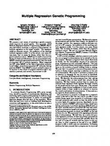
The principle of the crossover operator is schematised in Figure 3 using the expression already introduced. The crossover O: V × V→V, between two parse trees, x1, x2 ∈ V, can be defined through the following pro-

The crossover operator The principal inspiration for the formulation of crossover in GP arises from the biological practice of sexual reproduction. Similarly to what occurs in dip-

cedure:

• • •

select a node, n1, randomly in the tree x1; select a node, n2, randomly in the tree x2; interchange the two sub-trees.

loidal reproduction, the action of crossover affects two parental entities’ genotypes and recombines them in to produce offspring genotypes. Thus the cross-

Mutation

over operator O affects two evolving entities in such a

Mutation, m, is a unary-type transformation that alters the

way that O: V × V→V. Effectively, the crossover operator

individual v ∈ V such that m: V→V. Each evolutionary-

represents a higher-order transformation of parental

algorithmic technique defines mutation in a sense that

entities.

best suits its own purpose. Biologically speaking, mutation

In principle, crossover requires that two ‘parent’

denotes a haploid, asexual manipulation of the genome.

expressions are divided and recombined into two offspring

Traditionally, in genetic algorithms, mutation is referred

expressions. The representations of the expressions that

to as ‘bit-flipping’, or a segment-inverting operation

are undergoing recombination must be such that the

(Babovic 1993, 1996). In evolutionary programming, a

47


|



Table 5

3.

|

|

02.1

|

2000

Pseudo-code for a mutation.

Constant-mutation, similar as above but now a constant will be selected and mutated by using some white noise.

4.

Inversion-mutation, which inverts the order in which operands are ordered in an expression in a random way; thus f(x1, x2, x3) might become, for example, f(x3, x1, x2).

Figure 3

|

The action of the crossover operator: the upper part of the figure illustrates parents that are selected for reproduction, and the lower part of the figure illustrates the offspring that are generated after crossover.

5.

Edit-mutation, which edits the parse tree based on semantic equivalence. This mutation does not alter the phenotype (the function computed) but just produces an equivalent smaller formula. An example of edit-mutation is to replace all occurrences of

mutation is understood as any manipulation of a structure (Fogel 1992). Evolutionary strategies use the term to describe a variety of different operators (Schwefel 1981). In genetic programming, however, the action of the mutation operator has frequently been described as a random substitution of a sub-tree with another sub-tree. There are several kinds of (computational) mutations possible. Some examples are: 1.

Branch-mutation, where a complete sub-tree is replaced with another, and in principle, arbitrary sub-tree that can be generated by one of the

(0 + x) in a parse tree with x. Both the crossover and mutation operators try to balance the heredity and variability components of the algorithm. Much research has investigated the influence of specific crossover and mutation schemes with respect to these two criteria. In the system that is being developed through these pages, the following algorithm outlined in Table 5 is used. In the present example, the algorithm is employed with two randomly chosen ‘parents’ from the 15% of survivors of the generation gap as described above.

initialisation methods described above. 2.

Node-mutation, which applies a ‘random’ change to a single node, replacing its original value by another

Soft brood selection

and, again in principle, arbitrary value. In the case

It might be clear from the previous discussion that cross-

of constants, it’s value is often slightly altered by

over and mutation are randomised methods that are likely

using some white noise.

to produce rather erroneous formulae from time to time.

48


|


Therefore, it might be worthwhile to detect such formulae


Table 6

|

1994), when one or two parent formulae are chosen to produce offspring, more offspring than will actually be inserted in the population will be generated using crossover and mutation. Subsequently a culling function will be used to determine which offspring will be inserted in the population. This culling function often takes the form of the same objective function that is used overall, with the difference that it will use only a tiny fraction of the data. This culling function is then a computationally cheap method to assess the worth of the offspring. This way early detection of bad offspring can be enforced and less computational effort is spent on evaluating these offspring. Soft brood selection is not used in our running example.

Determination of the stopping criterion An evolutionary algorithm is in principle an infinite iteration. In practice however, the run needs to be stopped at a certain point. Two methods of stopping a run may be used: stop after a certain number of generations, or stop

02.1

|

2000

Description of experiment.

early before spending too much effort in evaluating them on the entire data set. In soft brood selection (Tackett

|

Find Bernoulli’s Law of Energy Objective

Conservation

Terminal set

{z, v, p, R}

Function set

{ + , *, − , /, power}

Population model

Panmictic, generational, elitist

Selection method

Truncation selection

Truncation percentage

15%

Population size

500

Initialization method

Grow method on size

Initial size of formulae

15

Crossover rate

100%

Branch mutation rate

10%

Constant mutation rate

10%

Constant mutation magnitude

5%

Maximum size of formula

71

Stopping criterion

2 minutes of processing time on a Pentium 233 MHz computer

after a certain length of wall-clock time has passed. In the Bernoulli example the latter was chosen: a run is stopped after 2 minutes of optimisation.

genetic programming was not able to find the proper Summary of the parameter settings

formula. The best formula produced over 30 runs was (in

So far several parameters have been introduced. These

simplified form):

parameters define a reasonable genetic programming system. One of the properties of most evolutionary algorithms is that they are very robust in the precise parameter settings. Small, or sometimes even large, changes in the parameters have only a very small effect in the optimisation capabilities of the system. Table 6 describes the experiment.

This formula had a RMS error of 1.71 metres. There are a few reasons as to why the genetic programming system was not able to find the optimal formula. This has mainly to do with the magnitude of the numerical values and the dimensions the problem is stated in. The pressure variable for instance is stated in a numeric magnitude of 104, while

Results

the other variables and the desired output have a magnitude around 10. As the generation of constants adopted is

The genetic programming system was run 30 times with

also biased towards smaller values, it is difficult for the GP

different initial random seeds. Unfortunately, in this setup,

system to scale the pressure variables to workable values.

49


|



|

02.1

|

2000

A second, related, problem is that the problem is

and practicable empirical equation. GP lends itself quite

stated using particular units of measurement. The formula

naturally to the process of induction of mathematical

produced by GP does not take these into account and thus

models based on observations: GP is an efficient search

renders a dimensionally incorrect formula. On the surface

algorithm that need not assume the functional form of the

it seems that by scaling the inputs and outputs the problem

underlying relation. Given an appropriate set of basic

would be cast in dimensionless and commensurable terms,

functions, GP can discover a (sometimes very surprising)

thus removing the problems encountered in this exper-

mathematical model that approximates the data well. At

iment. In fact, regression techniques rely on such a scaling.

the same time, GP-induced models come in a symbolic form that can be interpreted by scientists (see, for example, Babovic 1996). However, the application of standard GP in a process

Conclusion for the Bernoulli experiment

of scientific discovery does not always guarantee satisfac-

In one sense the experiment failed: this genetic program-

tory results. Extensions of standard GP as described pre-

ming system was unable to find the Bernoulli equation in

viously in this text have been an object of several studies

any of the 30 runs. As it is generally more insightful to

(see, for example, Davidson et al. 1999). In certain cases,

consider failures than successes, this presents the oppor-

GP-induced relations are too complicated and provide

tunity to learn something. First, it was identified that the

little new insight on the process that generated the data.

problem lies mostly in the scaling and, more generally, in

One may argue that GP, in such situations, blindly fits

GP’s inability to handle units of measurement. Secondly,

parse trees to the data (in almost the same way as in Taylor

the parameters were set at some general values, not opti-

or Fourier series expansion). It can be argued that GP then

mised for the particular problem at hand. In (symbolic)

results in a model with accurate syntax, but with meaning-

regression one usually does not approach a problem with

less semantics. In these cases, the dimensions of the

such an all-or-nothing attitude, but rather one looks at the

induced formulae often do not fit, pointing at the physical

results from one or more runs, changes some settings (by

uselessness of induced relations.

for instance adding or removing variables or enlarging or restricting the function set) and performs some more runs. With this strategy very good results can be obtained with this technique. But keep in mind that when using a randomised technique such as GP, your mileage may vary.

UNIT TYPING IN GP

another

The present work is based on an augmented version of

approach to GP that provides better results with problems

GP – dimensionally aware GP – which is arguably more

involving units of measurement. This approach transcends

useful in the process of scientific discovery (Keijzer &

the level of symbolic regression towards the arguably

Babovic 1999).

The

following

sections

will

introduce

more useful goal of model induction. With this approach the Bernoulli equation problem was successfully solved (consult Keijzer & Babovic (1999) for details).

Nature of measurements Throughout science, the units of measurement of observed phenomena are used to classify, combine and manipulate

GENETIC PROGRAMMING FOR SCIENTIFIC DISCOVERY

experimental data. Measurement is the practice of applying arithmetic to the study of quantitative relations. Every measurement is made on some scale. According to Stevens

Engineering data, in most cases, cannot attain their

(1959), to make a measurement is simply to make ‘an

maximum usefulness until they are connected by a reliable

assignment of numerals to things according to a rule–any

50


|



|

02.1

|

2000

rule’. There is a close connection between the concept of a

The derivative scales D1 and D2 are similar if and only

scale and the concept of an application of arithmetic.

if they are defined on the basis of the same physical law,

Different kinds of scales represent different kinds of appli-

expressed with respect to the same classes of similar

cation of arithmetic. Units of measurement are the names

scales. Thus for example, the ‘kg m s − 2’ and the ‘ft lb s − 2’

of these scales. Simple unit names such as ‘kilogram’,

scales of force are similarly defined. From this follows a

‘second’, ‘°C’ are used for fundamental and associative

straightforward theorem that similarly defined derivative

scales. Complex unit names, such as ‘kg m s

−2

’ are used

for derivative scales.

scales are similar to each other. This theorem (proved by Ellis 1965, p. 133) is important because it implies that classes of similarly defined derivative scales are simply classes of similar scales and hence may serve as reference classes for the expression of numerical laws in the

Nature of derivative measurement Derivative measurement is a measurement by means of constants in numerical laws. Let us more precisely define this concept through consideration of a system A1, to be any system that meets certain specifications, and suppose that:

standard form of the equation as introduced in the sequel. A second important theorem reads as follows, let: k = f(l, t, m, . . .)

(13)

be a numerical law expressed with respect to the classes of (12)

similar scales (L), (T), (M), . . . , where k is the only system

is a numerical law which is found to be obeyed by all

to the law of the kind given in Equation (13) as a law

systems of the class (A). At the same time l1, t1, m1, . . . , are

expressed in the standard form. Then the theorem states

the results of any simultaneous measurements made on

that:

k1 = f(l1, t1, m1, . . .)

the system A1 on any scales of the classes of similar scales (L), (T), (M), . . . . Let us suppose further that k1 is a

or scale-dependent constant that appears. Let us also refer

Any law expressed in the standard form must be of the form

system-dependent constant and that if the systems of the class (A) are arranged in the order of this constant they are

k = Cla tb mc . . . ,

(14)

also arranged in the order of some quantity d which is known to be possessed by this system. The conditions for

where C, a, b, c, . . . , are constants which are neither

saying that we have a scale of measurement of d are then

system dependent nor scale dependent (see Ellis 1965,

clearly satisfied. Hence, we may take k1 to be the measure

pp. 204–206).

of the quantity d which is possessed by the system A1 on a

The importance of this theorem is that it enables us to

derivative scale that depends on the choices of scales from

explain complex unit names and dimensional formulae.

within classes (L), (T), (M), . . . . Derivative measurement

Thus Equation (14) defines a class of similar derivative

of a quantity d is possible, therefore, if and only if there

scales for the measurement of some quantity d. To

exists some numerical law relating to the system that

designate this class we could use a simple name, say ‘N’,

possesses the quantity d in which there appears a system-

but it is obviously more informative to use the dimensional

dependent constant such that if these systems are

formula (L)a (T)b (M)c, . . . . By doing so, we say something

arranged in the order of this system-dependent constant,

about the form of the law (14) on which our derivative

they are also arranged in the order of d. A derivative scale

scales are defined.

for the measurement of d is then one that is defined by

The theory of dimensional analysis cannot be devel-

taking the value of the system-dependent constant (or

oped here, but its power depends on the information we

some strictly monotonic increasing function of it) for some

pack into dimensional formulae. If we wish to increase

particular choice of independent scales as the measure of

this power, we must include more information. This can be

the quantity d.

done only if we adopt the basic convention of expressing

51


|



|

02.1

|

2000

our laws with respect to the classes of similar scales. Thus

For example, v[1, − 1, 0] designates a variable, v, with a

instead of expressing laws, including angular displace-

derived dimension of velocity. User-defined constants

ment, with respect to the radian scale and saying

can be defined along with their dimensions, such

(absurdly) that angular displacement is a dimensionless

as 9.81[1, − 2, 0] defining the Earth’s gravitational

quantity, we should always express laws with respect to

acceleration.

the class of scales similar to our radian scale and introduce

Randomly generated constants are allowed only as

†

dimensionless quantities ([0, 0, 0]). There is a definitive

As demonstrated by Ellis (1965, pp. 145–151), this would

reason for allowing random numbers to be dimensionless

increase the power of dimensional analysis.

only. Should random constants with random dimensions

the dimension of angle into our dimensional formulae.

be allowed, GP would have an easy way of correcting the dimensions by introducing transformation from one

Introduction of units of measurements in GP

arbitrary unit of measurement to another. Some form of

To accommodate the additional information available

pressure should be applied to the application of unit

through units of measurement, the following extensions of

transformation.

standard GP were proposed (Keijzer & Babovic 1999). In the dimension-augmented setup, every node in the tree maintains a description of the units of the measurement it uses. These units (entirely in the spirit of the

Definition of the function set

standard form of Equation (14)) are stored as arrays of

Application

real-valued exponents of the corresponding dimensions.

augmented terminals violates the closure property for

In the present set of experiments only the dimensions of

these functions (Koza 1992). For example, adding metres

length, time and mass (LTM) are used, but the set up may

to seconds renders a dimensionally incorrect result of

be trivially extended to include all other SI dimensions

the operation. Therefore, the definition of arithmetic

(amount of substance, electric current, thermodynamic

operators is augmented to:

temperature and luminous intensity). Square brackets are used to designate units, for example [1, − 2, 0] corresponds to a dimension of acceleration (L1T − 2M0). Similarly, [0, 0, 0] defines a dimensionless quantity.

of

arithmetic

functions

on

dimension-

(1) specify the transformation of units of measurement; (2) accommodate units of measurement-related constraints on the application of functions; and (3) introduce a protection mechanism in order to satisfy the closure property.

Definition of the terminal set

Table 7 summarises the effects of the application of func-

The definition of the terminal set is straightforward, in

tions on units of measurement and specifies constraints on

that variables and constants are accompanied with the

the applications of functions. For example, exponentiation

exponents of their respective units of measurement. In the

of a value can only take place when the operand is

running example of the Bernoulli equation, this would

dimensionless, in which case the result of the operation is

read:

also a dimensionless value. Similarly, addition and subtraction are constrained so that their operands must have the same dimensions. Multiplication and division combine

T = {z[1, 0, 0], v[1, − 1, 0], p[ − 1, − 2, 1], g = 9.81[1, − 2, 0], g = 9810[ − 2, − 2, 1]}. †

(15)

Using radians as a separate dimension is not the end of the controversy. For the sake of argument let us introduce the quantity Q measured in radians. Let us also introduce two additional quantities P and R, measured in kilograms. Let us now calculate W = Q + arcsine (P/R). This would be syntactically perfectly correct, as the arcsine function would expect a dimensionless quantity while returning a value in radians. However, the derivative measurement of W is unacceptable.

the exponents by adding and subtracting the dimension exponents respectively. The standard Power function can be applied to dimensionless values only, whereas PowScalar can be applied to dimensional operands, affecting their dimensions correspondingly. Other functions can be defined in similar ways.

52


Table 7

|

|


Effects and constraints that units of measurement impose on the function set.

Function

Operand dimensionality

Result

Exponentiation:

[0, 0, 0]

[0, 0, 0]

Logarithm:

[0, 0, 0]

[0, 0, 0]

Square root:

[x, y, z]

[x/2, y/2, z/2]

Addition:

[x, y, z], [x, y, z]

[x, y, z]

Subtraction:

[x, y, z], [x, y, z]

[x, y, z]

Multiplication:

[x, y, z], [u, v, w]

[x + u, y + v, z + w]

Division:

[x, y, z], [u, v, w]

[x − u, y − v, z − w]

Power:

[0, 0, 0], [0, 0, 0]

[0, 0, 0]

PowScalar (c):

[x, y, z]

[x*c, y*c, z*c]

If less than zero:

[0, 0, 0], [x, y, z], [x, y, z]

[x, y, z]


|

02.1

|

2000

measurement to any other unit of measurement with such a multiplication. For an example of this operation, consider the addition function that receives one argument stated in metres and another argument stated in seconds. As such it is an undefined operation. It is however possible to transform the first argument to seconds by multiplying it with a constant of magnitude 1, stated in seconds per metre, or, equivalently, multiply the second argument with a constant of magnitude 1 stated in metres per second. A third possibility is to render both arguments dimensionless. Although at first sight, it may appear that this method eliminates all the problems related to dimensions, it is evident that this method ‘fixes’ any dimensionality-related problem by introducing physically meaningless transformations into evolving formulae. As such this method does not contribute anything to standard GP. To help the system find dimensionally correct formulations, a second objective next to the common goodnessof-fit criterion is employed. This objective takes full advantage of the explicit representation of the dimensions as a vector of real valued exponents. Define the distance of

Closure and strong typing The definition of the function and terminal set as it stands

an expression between a dimensionally correct formulation and its dimensional ‘fix’ to be the sum of all these arbitrary transformations as:

violates the closure property (Koza 1992). The closure property requires that each of the functions in the function

Goodness-of-dimension = ∑(zxiz + zyiz + zziz), (16)

set be able to accept, as its arguments, any value and data type that may be returned by any function, and any

where the subscript i ranges over all transformations

value and data type that may possibly be assumed by

applied to the formula, and x, y and z are the components

any terminal.

of the corresponding dimension vector. This goodness-of-

This problem was already encountered in symbolic

dimension acts as an effective measurement of distance

regression where the division function as such violates the

from desired dimensions and is treated as an additional

closure problem. One of the methods to enforce closure

measure of fitness. Goodness-of-dimension can be com-

was to protect such functions. In the unit augmented

bined with the goodness-of-fit statistic in a multi-objective

version of genetic programming this path is taken.

optimisation fashion.

The functions in this system are protected so that

It is however also possible, at the expense of a rather

whenever incompatible data types are encountered as

large modification, to modify the present approach and

arguments to a function, the arguments are multiplied

include dimensional constraints more strongly. One can

with a constant of magnitude 1.0 whose unit of measure-

adopt strict admissibility and admit only those formu-

ment is such that it will transform the argument’s unit to

lations that are dimensionally correct. Montana (1995)

the desired unit. Because of the particular structure of the

proposed a so-called strongly typed genetic programming

dimension equations, it is possible to transform a unit of

system (STGP) where the closure property is not enforced,

53


|



|

02.1

|

2000

but rather the system is constrained so that data types are

correspondence between the model and the real world.

respected and only well-formed expressions are ever

Parameters of this sort serve in effect as error compen-

created. This solves the problem of a naı¨ve implemen-

sation devices that artificially adjust the model results to

tation where expressions that violate the typing scheme

compensate for the fundamental discrepancies that exist

are destroyed. In such a naïve setting the number of

between the real world and its representation within the

ill-formed expressions (the ones with goodness-of-

model. Chezy’s C is much more than a coefficient that can

dimension larger than zero) is very likely to be large. It is

be associated with roughness forces only, and as such is

consequently very likely that the system will spend most of

not well-defined in nature. Instead it exists only at the

its time creating, evaluating and dismissing solutions,

interface between nature and model. It has to accommo-

which is not far from a random walk.

date both: a part related to physical processes, but also a

Consequently the mechanism proposed here is not a

part that has to do with our schematisation of nature

form of strongly typed GP as it does maintain the closure

within a model. One may even ask ‘What is the physical

property through a protection mechanism. A strongly

meaning of such a parameter—how well is it grounded, and

typed GP would initialise and keep all expressions dimen-

indeed is it grounded at all?’ We may be able to read a

sionally correct throughout the evolutionary process. For

certain ‘physical meaning’ into such calibration par-

ill-posed and incomplete problems (for example the ones

ameters, but they do not exist as such and are thus ‘dis-

in which one of the observations is not supplied), a

connected’ in a fundamental way from the world that they

strongly typed GP would fail even at initialisation. The

are supposed to model (Minns & Babovic 1996).

adopted, weakly typed approach allows dimensionally

At the same time, it is quite obvious that the

incorrect solutions that are repaired at run-time. At

dimensions of such calibration coefficients are chosen in a

the same time, evolutionary pressure on dimensional

way that the overall dimension within a model will match.

incorrectness is added through a supplementary objective.

As such, they may have little physical meaning.

The present version of GP is therefore based on a prefer-

Strongly typed GP would only reinforce such a

ence towards dimensional consistency rather than an

position and that may not be the most appropriate one for

enforcement of this quality.

the process of scientific discovery. If we are to design an

It is believed that this version of GP may be more

algorithm that can be truly useful in a process of scientific

appropriate in the process of scientific discovery. Let us

discovery, we have to be able to utilise all the available

accept it—science is packed with ‘magical numbers’ (for

information (including units of measurements) and

example, the Kolmogorov–Obukhkov 2/3 exponent,

possibly extend upon it.

which is a constant source of controversy in turbulence modelling). Dimensions of some of these coefficients are everything but transparent. For example, the Chezy number, at the very centre of this study has dimensions of

Dimension-based brood selection

m1/2 s − 1 and is still referred to as a roughness coefficient!

An alternative brood selection is applied in this system

The fact is that the Chezy number, C, allows for a range of

(Keijzer & Babovic 1999). In this case the culling function

phenomena not explicitly taken into account in the well-

used in dimensionally aware GP is the goodness-of-

known formula defining average flow velocity in steady

dimension of a formula. This evaluation is very inexpen-

conditions:

sive as it can be calculated independently of the training

u = C' (Ri).

set and it requires a single pass through the parse tree. (17)

The

present

implementation

reads

as

follows:

two parents are chosen for crossover; they produce m

Since functional similarity to the natural system is sup-

offspring by repeated application of the random sub-tree

posed to be comprehended by the equation itself, it is this

crossover operation; constraint violations are corrected

calibration coefficient C that then must capture the exact

for dimensions in the manner outlined above; and, finally,

54


|



|

02.1

|

2000

the best among the m offspring with respect to goodness-

if highly parameterised), model is used as a source of

of-dimension are added to the intermediate population.

data that are then further processed by two apparently different methodologies in order to induce a more compact model of the additional bed resistance caused by vegetation.

ADDITIONAL RESISTANCE TO FLOW INDUCED BY FLEXIBLE VEGETATION Based on the bitter experiences of recent floods in Europe

Short description of the Kutija-Hong model

and the USA, many pressure groups have promoted the

As indicated earlier, the Kutija-Hong model is based on a

restoration of natural wetlands that would act as natural

differential equation of the conservation of momentum in

‘sponges’ capable of absorbing excess water and thus

the horizontal direction:

reducing flooding risks. Various governments around the world (The Netherlands, USA, etc.) have embarked on major wetland protection and restoration tasks. This

where:

accelerating movement to restore wetlands, and especially

u denotes horizontal velocity

to return flood plains to more natural conditions, has lead

w denotes vertical velocity

to the widespread introduction and propagation of reeds

P denotes pressure

and other forms of more or less flexible vegetation. These

r denotes density of water

reeds and other plants then influence flows across wet-

g denotes gravity acceleration

lands. The need to control flooding events and intensity

i

using numerical models and other tools necessitates a

denotes bottom slope

t denotes shear stress

better understanding of the influence of this type of

and the term Fx/rxz represents the additional specific

vegetation on flow.

drag forces.

The wetland restoration projects favour the growth of

The model is developed to address the effects of

reeds and other similar vegetation within a river basin.

flexible vegetation in steady flow conditions only, so the

The presence of vegetation influences the flow conditions,

convective momentum terms and pressure term are

and in particular the bed resistance, to a large degree.

neglected. The numerical model is based on a finite differ-

However, the influence of the rigid and flexible vegetation

ence implicit approximation for the unknown velocities at

on flow conditions is not understood well enough. The

the discretisation points.

present work is concerned with the understanding and

The model takes into account the effects of shear

formulation of the underlying physical processes. Some

stresses on the bed and the additional forces induced by

laboratory experiments using physical scale modelling

flow through vegetation, and it possesses a facility to adapt

have been performed (Larsen et al. 1990; Tsujimoto

initial distributions of velocities over discretisation points

et al. 1993), but only over a limited range and with

on the vegetation stems. In addition to representing these

variable success. Similarly, although field experiments are

influences, the model takes into account the bending of

continuing, the data available remains scarce.

the reeds under the loads produced by the drag forces.

More recently, a numerical model has been developed

Owing to bending, the effective reed height is reduced,

with the intention of deepening the understanding of the

which implies a lesser drag, and this in turn implies a

underlying processes (Kutija & Hong 1996). This model is

reduction in the drag-induced deflections of the veg-

a one-dimensional vertical model based on the equations

etation. These processes are resolved through an iterative

of conservation of momentum in the horizontal direction.

numerical process. For a more detailed description and a

This numerical model is employed here as an experimental

discussion of the specifics of the model see Kutija & Hong

apparatus in the sense that this, fully deterministic (even

(1996).

55


|



|

MODEL INDUCTION

Table 8

Data

(/ (exp (−d hr)) (−(rlog (/ (rlog (/ m hw)) (sqrt (sqrt (/ d d))))) (* (/ hr (sqrt (sqrt (/ d (sqrt (sqrt (exp (−d hr)))))))) (* (* (rlog (/ (rlog (/ m hr)) (exp (−d hr)))) (* (−(−d hr) hr) −0.00410)) p))))

The Kutija-Hong model, used as a generator of data, was in effect used as a truthful representation of a physical reality, while providing the conveniences of fast calculation and an ability to produce results with any degree of scale refinement. In this way, the numerical model not only replaced physical scale modelling facilities within

|

02.1

|

2000

The best performing expressions for the dimensional case (Babovic 1996).

this exploratory environment, but also introduced several intrinsic advantages over scale models. It is well known that so-called roughness scaling is one of the principal difficulties in the development of physical models. Since the roughness is the primary phenomenon in question here, the issue of its physical correctness remained critical. The ‘realism’ of the complete numerical model was

Results obtained using genetic programming Previously reported work

reasonably well proven against experimental data in the

The following two sections are adapted from Babovic

case of stiff (non-flexible) vegetation (Kutija & Hong

(1996) and Babovic & Keijzer (1999). In the first instance,

1996).

a standard genetic programming environment has been set

The model has been run with a wide range of input

up. The results of Kutija-Hong simulations were presented

parameters in order to create training data. As the first

as Cnew: the Chezy number corresponding to the flow

attempt towards the development of a model of additional

conditions with developed vegetation.

roughness, only the effects of non-flexible reeds with high

Dimensional values

stiffness were simulated. Altogether, some 4,800 items of

In the first attempt, all the data were used in their original,

training data were generated. The training data consisted,

dimensional form. Such an approach was adopted so as to

in the first instance, of dimensional numbers formed from:

introduce the least possible level of ‘presuppositions’

• • • •

water depth hw,

in the model evolution. From the perspective of

•

numerical parameter p related to the eddy-viscosity

reed height hr, reed diameter d, number of individual reed shoots per square metre m, approximation and its further relation to the vegetated layer height.

accuracy (goodness-of-fit), the obtained results were quite satisfactory (see Table 8). The shear complexity of the formulation above almost immediately eliminates it from a knowledge induction framework. In order to improve interpretability, Babovic & Keijzer (1999) employed an early version of dimensionally aware GP with the best performing formula being:

The input data varied in the ranges: 2.5 ≤ hw ≤ 4.0 0.25 ≤ hr ≤ 2.25 50 ≤ m≤ 350 0.001 ≤ d ≤ 0.004 0.4 ≤ p ≤ 1.0

There is some dispersion for the higher values of Cnew but otherwise the equation exhibits good accuracy (see Table 9). The scatter plot for Equation (19) is depicted in Figure 4. However, it has to be emphasised that Equation (19) is not dimensionally correct. This shortcoming can be

56


Table 9

|

|


r

R

(19)

0.96

(25)

0.94

|

02.1

u = hC' (Ri) .

Statistical summary for expressions (19) and (25). 2


RMS

NRMS

0.92

2.880

27.89%

0.89

0.076

37.47%

|

2000

(20)

For example, for h = 0, the resistance to flow becomes infinitely large, thus stopping the water flow, which is, physically a highly unlikely situation. The smallest values of h experienced with the Kutija-Hong numerical model were h 0.1. For h = 1, the influence of vegetation on the roughness is zero. Another set of model induction experiments has been performed, but in this case a collection of dimensionless

corrected by introducing an auxiliary constant with

numbers has been used. The dimensionless ratios intro-

dimension of length and magnitude of 1.0 that should be

duced were defined as follows:

multiplied with dimensionless p to correct dimensions. At the same time, both constants 55.93 and 11.39 should be

hrel = hw/hr;

(21)

wd = hw/d;

(22)

rd = hr/d;

(23)

hhwhrd = (hw − hr)/md.

(24)

assigned dimensions of the Chezy number [m1/2 s − 1] to make this formula dimensionally correct. As indicated earlier, such behaviour is not surprising when applying standard instances of GP. Satisfactory goodness-of-fit may be obtained, but the semantics of the generated expressions cannot be warranted. Dimensionless values One standard approach in avoiding potential conflicts

In addition to these, parameters p and m were used

with incorrect dimensionality of induced formulations

without any changes. The best performing expression is:

is to use dimensionless values. This is a ‘standard scientific practice’. Units of measurements are effectively eliminated through the introduction of dimensionless ratios. Once the dimensionless numbers are used instead of the original dimensional values the problem of

The performance statistics are presented in Table 9.

dimensional correctness is conveniently avoided, as all

Where:

analysed quantities are dimension-free. It is also argued

r

denotes correlation coefficient,

that dimensionless ratios collapse the original search

R2

denotes Pearson’s product moment correlation

RMS

denotes Root Mean Squared Error,

space, making it more compact, thus resulting in a more effective behaviour of algorithms that fit models

squared,

to the data. At the same time, the information contained

NRMS denotes Normalised Root Mean Squared Error

in the units of measurements is ignored entirely,

where RMS is normalised by the standard deviation of the

effectively violating the basic premise of dimensional

desired outcome (Kutija-Hong model in this case).

analysis.

The first interesting observation is slightly counter-

In this, dimensionless case, the results of Kutija-Hong

intuitive: the accuracy of induced formulation in a

simulations were presented as a dimensionless ratio h of

dimensionless case is not as good as the accuracy of

an original Chezy number, that corresponding to an

dimensional formulation. Even if the accuracy of h

absence of vegetation, and a new Chezy number, that

would be acceptable, it is the behaviour of Chezy’s C

corresponding to developed vegetation. This ratio h can

(calculated as Cnew = hCorg) that is highly undesirable

be conveniently incorporated in the Chezy formula for

in this case (see the upper two graphs in Figure 4).

velocity under steady flow conditions:

Compression of the search space through the use of

57


Figure 4

|

|



|

02.1

|

2000

Scatter plots for expressions (19), (25) and (26). The upper two graphs depict the behaviour of an induced relation in the dimensionless case (denoted as FDL). The graph in the upper left corner is a scatter plot for dimensionless h, whereas the graph in the upper right corner is a plot for the corresponding Chezy coefficient. The graph in the lower left corner depicts performance in the dimensional case (FDM). Finally the graph in the lower right corner depicts the results for the dimensionally aware GP (FDAGP).

dimensionless values obviously incorporates several

sponding

hidden risks that need to be handled with considerable

measurements. The purpose for conducting such an

care.

experiment was to test whether such a dimensionally

dimensionless

parameters

based

on

the

aware GP setup is capable of creating a dimensionally correct and still accurate formulation. Since the preResults based on dimensionally aware genetic

processing of raw observations was not employed here, it

programming

can be argued that GP was confronted with a problem of trying to formulate a solution from first principles. The

By way of comparison, a dimensionally aware genetic

evolutionary processes resulted in a number of expres-

programming environment was set up in such a way as

sions, of which only the most interesting one is presented

to comprehend all measured data and not the corre-

here:

58


Table 10

|

|



r

R

(19)

0.96

(25) (26)

02.1

|

2000

this direction must resolve this deficiency in one way

Statistical summary for expressions (19), (25) and (26). 2

|

RMS

NRMS

0.92

2.880

27.89%

0.94

0.89

0.076

37.47%

0.98

0.97

1.800

17.44%

or another. 2.

Another possibility may be that the problem is simply ill-posed: the authors attempted to model Chezy’s C despite their reservation about its grounding (however, without any reservations about its usefulness).

The authors maintain that this particular approach is very useful for the purposes of model induction. This dimensionally aware attitude is open-ended in that it does not strictly adhere to the dimensional analysis framework. Such an approach provides the possibility of achieving a superior goodness-of-fit while sacrificing goodness-ofThe degree of accuracy of the induced expression is quite

dimension (while obtaining good performance in both

satisfactory. A statistical measure of conformity, such as

objectives). The authors will go even further to claim that

the Pearson’s R2, gives a value of 0.97. This provides a

the dimensionally aware approach is much more useful

considerable improvement over the values of 0.92 or 0.89

than a strict use of dimensional analysis to create and use

based on the relations described in Equations (19) and

only dimensionless ratios.

(25) respectively. The total error over the data set is

At the same time, the authors remind the reader that

reduced and all other statistical measures of accuracy

the object of the presented exercise is to find an empirical

disclose improvements (see Table 9 and Table 10 for

equation based on data. The present work cannot be

details).

characterised as a search for a universal law (though it

At the same time the formula is dimensionally consist-

might help). The rationale of this approach is to utilise

ent, it uses some of the most relevant physical properties

whatever information is available, yet not to bias this

in the relevant context. For example, the dimensionless

search too strongly. Being able to use units of measure-

term (hw − hr) p/dm describes a ratio between the effec-

ments (either through the dimensionally aware or

tively available cross-section (hw − hr) p and a part of the

through strong adherence to dimensional analysis) pro-

cross-section that is blocked by the plants per unit width

vides an opportunity to truly mine the knowledge from

of the channel.

the data, to learn more from data and other associated

The remaining group g/hrY represents a ratio of

gravity forces and flow resistance ‘force’ expressed through the reed height.

information. One open question still remains: what to do with the proposed formulae? Fortunately, the primary purpose of

In the present case, evolution produced a dimension-

this text (in the light of the previous discussion) is not to

ally consistent, meaning-rich formulation that is very ac-

propose a formulation for the additional resistance to flow

curate. It did so without employing assumptions (other

induced by vegetation, but to demonstrate an alterna-

than units of measurement); the process operated only on

tive discovery process. The physical interpretation of

raw observations. Still, Equation (26) is not dimensionally

Equations (19), (25) and (26) requires a wealth of knowl-

correct; it does not produce the derived units for the Chezy

edge in flow retardance and hydraulic resistance. The

coefficient. This may originate in at least two causes:

authors feel that such a discussion would fall outside the immediate scope of the present paper.

1.

Incomplete data: in the present data set neither time

Thus, the final proposal of the best formula is not even

nor elasticity components were provided (the

attempted here. Such a choice should be made by the

authors supplied g = 9.81 m/s2). The next iteration in

experts in the field, by the people who can competently

59


|



|

02.1

|

2000

judge the quality of the data sets used, interpret the

models that can be interpreted by the domain experts.

induced model and in the end choose the one that makes

Once a model is interpreted, it can be used with confi-

most sense. We would rather view such results as a poten-

dence. It is only in this way that one can take full

tial opening of a new research direction in this field (and

advantage of knowledge discovery and advance our

for that matter any other domain), so that we can talk

understanding of physical processes.

research.

Although the results presented here are based on

Domain experts can be exposed to a completely new set of

preliminary experiments, one main conclusion can be

formulations, off the beaten track, yet within the domain

drawn. Traditionally, dimensionless numbers are used as

of physical validity. Unfortunately, no physical exper-

the dominant vehicle in interpretation and modelling of

imental data were available for verification of the model.

experimental values. Such a choice is natural as this

Owing to this lack of experimental data, the authors invite

alternative conveniently avoids the issues related to

other researchers to check these models using their own

dimensional analysis and its correctness. It is also believed

data. The experts should make the ultimate step in this

that dimensional numbers collapse the search space and

process.

that resulting formulations are more compact. This paper

about

knowledge–discovery-driven

domain

Although no direct evidence has been offered in this

demonstrated that it can be advantageous to use data

work, a few concluding remarks need to be forwarded in

together with its dimensions. The knowledge–discovery

the favour of the performance of dimensionally aware GP.

software system uses this information to guide a search for

The convergence rate of such an augmented version of GP

an accurate and physically sound formulation. The result

is much better than the one in standard GP. The reasons

is more accurate than the one achieved when a more

for such a behaviour are fairly obvious: units of measure-

conventional approach is followed.

ment are taken into account as an additional objective so that this information also directs the search process. One may say that GP effectively spends more of its time on performing physically more sensible operations in an altered search space. At the same time, standard GP

ACKNOWLEDGEMENTS

often grows parse trees of a considerable size in order

The authors gratefully acknowledge Dr Vedrana Kutija

to meet goodness-of-fit criterion only. The interested

for the use of data. This work was in part funded by

reader is referred to Keijzer & Babovic (1999) for a direct

the Danish Technical Research Council (STVF) under

comparison of the two approaches.

the Talent Project No. 9800463 entitled ‘Data to

Fundamentally, augmentation of GP with dimensional

Knowledge—D2K’. Their support is greatly appreciated.

information adds a descriptive, semantic component to

For more information on the project visit http://

the algorithm. This is in addition to the functional

projects.dhi.dk/d2k.

semantics that define the manipulation on numbers. While functional semantics ground the formulae in mathematics, the dimensional semantics ground them in the physical domain.

REFERENCES

CONCLUSIONS The described work is part of a research effort aiming at providing new (and sometimes provocative) hypotheses built from data alone. The ultimate objective is to build

Abbott, M. B. 1993 The electronic encapsulation of knowledge in hydraulics, hydrology and water resources. Adv. Wat. Res. 16, 21–39. Babovic, V. 1993 Evolutionary algorithms as a theme in water resources. In Scientific Presentations, AIO meeting ‘93, pp. 21–36. Delft University of Technology. Babovic, V. 1996 Emergence, Evolution, Intelligence: Hydroinformatics. Balkema, Rotterdam.

60


|


Babovic, V. & Keijzer, M. 1999 Computer supported knowledge discovery—a case study in flow resistance induced by vegetation. In Proceedings of the XXVI Congress of International Association for Hydraulic Research, Graz, 1999. Bohm, W. & Geyer-Schulz, A. 1996 Exact uniform initialization for genetic programming. In Foundations of Genetic Algorithms IV (ed. R. K. Belew & M. Vose). University of San Diego, CA, USA, Morgan Kaufmann. Box, G. E. P. 1957 Evolutionary Operation—a method for increasing industrial productivity. Appl. Stat. 6, 81–101. Bremermann, R. M. 1958 A learning machine. IBM Jl Res. Dev. 2, 2–13. Cramer, N. L. 1985 A representation for the adaptive generation of simple sequential programs. In Proceedings of an International Conference on Genetic Algorithms and Their Applications (ed. J. J. Grefenstette), pp. 183–187. Davidson, J. W., Savic, D. & Walters, G. A. 1999 Method for the identification of explicit formulae for the friction in turbulent pipe flow. J. Hydroinformatics 1(2), 115–126. Ellis, B. D. 1965 Basic Concepts of Measurements. Cambridge University Press. Fayyad, U., Piatetsky-Shapiro, G. & Smyth, P. 1996 From data mining to knowledge discovery: an overview. In Advances in Knowledge Discovery and Data Mining (ed. U. Fayyad, G. Piatetsky-Shapiro, P. Smyth & R. Uthurusamy), pp. 1–36. MIT Press, Cambridge, MA. Fogel, D. B. 1992 Evolving Artificial Intelligence. Ph.D. thesis, University of California at San Diego. Fogel, D. B. 1993 Evolving behaviours in the iterated prisoner’s dilemma. Evolutionary Computation 1(1), 77–97. Fogel, D. B., Fogel, L. J. & Porto, V. W. 1990 Evolving neural networks. Biological Cybernetics 63(6), 487–493. Fogel, L. J., Owens, A. J. & Walsh, M. J. 1966 Artificial Intelligence Through Simulated Evolution. Ginn, Needham Height. Foseca, C. M. & Fleming, P. J. 1995 An overview of Evolutionary Algorithms in Multiobjective Optimization 3(1), 1–16 Friedberg, R. M. 1958 A learning machine. IBM Jl Res. Dev. 2, 2–13. Goldberg, D. E. 1989 Genetic Algorithms in Search, Optimisation and Machine Learning. Addison Wesley, New York. Grefenstette, J. 1997 Proportional selection and sampling algorithms. In Handbook of Evolutionary Computation (ed. D. Back, B. Fogel & A. Michalewicz), C2:2:1. Oxford University Press. Harvey, I. 1993 Artificial Evolution and Adaptive Behaviour. Ph.D. thesis, University of Sussex, UK. Holland, J. H. 1975 Adaptation in Natural and Artificial Systems. University of Michigan, Illinois.


|

02.1

|

2000

Keijzer, M. & Babovic, V. 1999 Dimensionally aware genetic programming. In GECCO-99: Proceedings of the Genetic and Evolutionary Computation Conference, July 13–17, 1999, Orlando, Florida USA (ed. W. Banzhaf, J. Daida, A. E. Eiben, M. H. Garzon, V. Honavar, M. Jakiela & R. E. Smith). San Francisco, Morgan Kaufmann. Koza, J. R. 1992 Genetic Programming: On the Programming of Computers by Natural Selection. MIT Press, Cambridge, MA. Koza, J. R. 1994 Genetic Programming 2: Automatic Discovery of Reusable Programs. MIT Press, Cambridge, MA Kutija, V. & Hong, H. T. M. 1996 A numerical model for addressing the additional resistance to flow introduced by flexible vegetation. J. Hydraul. Res. 34(1), 99–114. Larsen, T., Frier, J. O. & Vestergraard, K. 1990 Discharge/stage relation in vegetated Danish stream. In International Conference on River Flood Hydraulics. Margalef, R. 1968 Perspectives in Ecological Theory. University of Chicago, Ill. Maynard Smith, J. 1975 The Theory Of Evolution. Penguin, London. Michalewicz, A. 1992 Genetic Algorithms + Data Structures = Evolution Programs. Springer, Berlin. Minns, A. W. & Babovic, V. 1996 Hydrological Modelling in a Hydroinformatics Context. In Distributed Hydrological Modelling (ed. M. B. Abbott & J. C. Refsgaard), pp. 297–312. Kluwer Academic Publishers. Minsky, M. 1963 Steps towards artificial intelligence. In Computers and Thought (ed. E. A. Feigenbaum & J. Feldman), pp. 379–384. McGraw Hill, New York. Montana, D. J. 1995 Strongly typed genetic programming. Evolutionary Computation 3(2), 199–230. Radcliffe, N. J. & Surry, P. D. 1994 The reproductive plan language RPL2: motivation, architecture and applications. In Genetic Algorithms in Optimisation, Simulation and Modelling (ed. J. Stender, E. Hillebrand & J. Kingdom), pp. 65–94. IOS Press, Amsterdam. Schwefel, H.-P. 1981 Numerical Optimisation of Computer Models. Wiley, Chichester. Stevens, S. S. 1959 Measurement, psychophysics and utility. In Measurements: Definitions and Theories (ed. C. W. Churchman & P. Ratoosh). New York. Tackett, W. A. 1994 Recombination, Selection, and the Genetic Construction of Computer Programs. Ph.D. thesis, University of Southern California. Tsujimoto, T., Okada, T. & Omata, A. 1993 Field measurements of turbulent flow over vegetation on flood plain of river Kakehaski. KHL Progressive Report, Hydraulic Laboratory, Kanazawa University.

Genetic programming as a model induction engine - CiteSeerX

Genetic programming as a model induction engine - CiteSeerX

Suggest Documents

Genetic Programming on Program Traces as an Inference Engine for ...

genetic programming based model structure identification ... - CiteSeerX

The Genetic Algorithm as a Discovery Engine - Cartesian Genetic ...

A Hardware Engine for Genetic Algorithms - CiteSeerX

Genetic Programming Reconsidered - CiteSeerX

A Genetic Programming System for the Induction of ... - Semantic Scholar

Genetic Programming for the Induction of Seasonal Forecasts: A Study

Map-reduce as a Programming Model for Custom ... - CiteSeerX

GAPS: a genetic programming system - Computer ... - CiteSeerX

Developmental Evaluation in Genetic Programming: A ... - CiteSeerX

Towards a Genetic Programming Algorithm for ... - CiteSeerX

A C++ Implementation of Genetic Programming - CiteSeerX

A Distributed Object-Oriented Genetic Programming ... - CiteSeerX

from Genetic Algorithms to Genetic Programming - CiteSeerX

Pattern-Guided Genetic Programming - CiteSeerX

Grammatically-based Genetic Programming - CiteSeerX

Parallel Distributed Genetic Programming - CiteSeerX

Pattern-Guided Genetic Programming - CiteSeerX

GENETIC PROGRAMMING TO DESIGN ... - CiteSeerX

Model-Driven Programming - CiteSeerX

Performance Enhanced Genetic Programming - CiteSeerX

Model-Driven Programming - CiteSeerX

Genetic Programming as an Analytical Tool for ... - CiteSeerX

The Genetic Algorithm as a Discovery Engine: Strange ... - Google Sites