Research
Genome-wide mapping and assembly of structural variant breakpoints in the mouse genome Aaron R. Quinlan,1 Royden A. Clark,1 Svetlana Sokolova,1 Mitchell L. Leibowitz,1 Yujun Zhang,2 Matthew E. Hurles,2 Joshua C. Mell,3 and Ira M. Hall1,4,5 1
Department of Biochemistry and Molecular Genetics, University of Virginia School of Medicine, Charlottesville, Virginia 22908, USA; Wellcome Trust Sanger Institute, Wellcome Trust Genome Campus, Hinxton, Cambridge CB10 1SA, United Kingdom; 3Department of Zoology, University of British Columbia, Vancouver, British Columbia V6T 3Z4, Canada; 4Center for Public Health Genomics, University of Virginia, Charlottesville, Virginia 22908, USA 2
Structural variation (SV) is a rich source of genetic diversity in mammals, but due to the challenges associated with mapping SV in complex genomes, basic questions regarding their genomic distribution and mechanistic origins remain unanswered. We have developed an algorithm (HYDRA) to localize SV breakpoints by paired-end mapping, and a general approach for the genome-wide assembly and interpretation of breakpoint sequences. We applied these methods to two inbred mouse strains: C57BL/6J and DBA/2J. We demonstrate that HYDRA accurately maps diverse classes of SV, including those involving repetitive elements such as transposons and segmental duplications; however, our analysis of the C57BL/6J reference strain shows that incomplete reference genome assemblies are a major source of noise. We report 7196 SVs between the two strains, more than two-thirds of which are due to transposon insertions. Of the remainder, 59% are deletions (relative to the reference), 26% are insertions of unlinked DNA, 9% are tandem duplications, and 6% are inversions. To investigate the origins of SV, we characterized 3316 breakpoint sequences at single-nucleotide resolution. We find that ;16% of non-transposon SVs have complex breakpoint patterns consistent with template switching during DNA replication or repair, and that this process appears to preferentially generate certain classes of complex variants. Moreover, we find that SVs are significantly enriched in regions of segmental duplication, but that this effect is largely independent of DNA sequence homology and thus cannot be explained by non-allelic homologous recombination (NAHR) alone. This result suggests that the genetic instability of such regions is often the cause rather than the consequence of duplicated genomic architecture. [Supplemental material is available online at http://www.genome.org. The sequence data generated for this study have been submitted to the Short Read Archive (http://www.ncbi.nlm.nih.gov/Traces/sra/sra.cgi) under accession no. SRA010027. Structural variant calls have been submitted to dbVAR (http://www.ncbi.nlm.nih.gov/projects/dbvar/) under accession no. nsdt19. Source code for the HYDRA algorithm is available at http://code.google.com/p/hydra-sv/.] In the six years since the first genome-wide analyses revealed extensive DNA copy number variation (CNV) among human individuals (Iafrate et al. 2004; Sebat et al. 2004), numerous studies have extended this observation in scope and scale with increasingly powerful genomic tools. It is now widely recognized that structural variation (SV), which includes duplications, deletions, inversions, transpositions, and other genomic rearrangements, is an abundant and functionally important class of genetic variation in mammals (Zhang et al. 2009a). Besides the emerging role of inherited variants in complex disease, new structural mutations contribute to sporadic human disorders, are a hallmark of tumor genomes, and drive the evolution of genes and species. For all of these reasons, it is important to generate accurate SV maps in many different organisms and cellular contexts, so that the biological consequences of SV may be assessed, and so that the molecular mechanisms that generate new variation may be fully understood. Several technical challenges have precluded a more complete understanding of the patterns and origins of SV. First, most studies have used array comparative genome hybridization (aCGH), which
5
Corresponding author. E-mail
[email protected]. Article published online before print. Article and publication date are at http://www.genome.org/cgi/doi/10.1101/gr.102970.109.
has limited resolution, cannot detect balanced rearrangements or reconstruct locus architecture, and has limited ability to detect SVs composed of multi-copy elements such as segmental duplications (SDs) or transposable elements (TEs). Second, sequence-based methods such as paired-end mapping (PEM) have emerged as a potent alternative to aCGH (Raphael et al. 2003; Tuzun et al. 2005; Korbel et al. 2007; Lee et al. 2008), but their practical utility has been limited by the high cost of ‘‘long-read’’ sequencing, and the computational difficulties associated with interpreting ‘‘short-read’’ sequence data from complex genomes. Thus, while a number of PEMbased algorithms have been developed to identify SV from shortread sequence data (Chen et al. 2009; Hormozdiari et al. 2009; Korbel et al. 2009; Medvedev et al. 2009) and newer methods have been devised to map SVs at higher resolution (Lee et al. 2009; Sindi et al. 2009), all short-read PEM studies except one (Hormozdiari et al. 2009) have restricted their analyses to paired-end reads that map uniquely to the reference genome. This approach is not ideal given that SVs often involve repeated sequences such as segmental duplications and transposons. Finally, it has been difficult to evaluate structural mutation mechanisms in an unbiased way because genome-wide studies have thus far characterized relatively few breakpoints at single-nucleotide resolution (Korbel et al. 2007; Kidd et al. 2008; Kim et al. 2008; Perry et al. 2008), and the relative contribution of different molecular mechanisms remains a matter of debate.
20:623–635 Ó 2010 by Cold Spring Harbor Laboratory Press; ISSN 1088-9051/10; www.genome.org
Genome Research www.genome.org
623
Quinlan et al. Despite rapid advances in DNA sequencing technologies, affordable and accurate assembly of entire mammalian genomes remains years away. Indeed, even traditional methods have difficulty resolving complex genomic regions. In the interim, we argue that the optimal solution for breakpoint detection is a hybrid approach that combines PEM and local de novo assembly. Here we describe a general approach for unbiased detection, assembly, and mechanistic interpretation of SV breakpoints using both short and long reads, and apply it to whole-genome sequence data from two widely used inbred mouse strains. We show that our algorithms accurately identify diverse classes of SV, capture an unprecedented number of variants, and reveal novel breakpoint features. Of mechanistic significance, we report an abundance of complex SVs that appear to be derived from template switching during DNA replication or repair, and a propensity for duplicated genomic regions to generate new variants through mechanism(s) other than non-allelic homologous recombination (NAHR). A unique strength of this study is our choice of the mouse genome; because the reference genome is derived from an established inbred line (C57BL/6J), we were able to sequence an animal whose genome should be essentially identical to the reference. This important methodological control, which has not been present in any other PEM study, allowed us to distinguish true genetic variation from technical ‘‘noise’’ and poorly assembled genomic regions.
Results Sequence data The sequence data for this study come from two independent sources (Table 1). First, we used Illumina paired-end sequencing (Bentley et al. 2008) to generate roughly 130 million and 75 million paired-end reads (which we refer to as ‘‘matepairs’’) each from the DBA/2J and C57BL/6J strains (hereafter referred to as DBA and B6, respectively). Matepairs had a median fragment size of 432 and 457 bp, resulting in 13.4 and 8.3 mean physical coverage for DBA and B6, respectively (Supplemental Figs. S1, S2; Table 1). We aligned reads with the BWA algorithm (Li and Durbin 2009), which identified ;88% of DBA and 95% of B6 matepairs as ‘‘concordant,’’ meaning that they mapped to the reference genome with the expected orientation and size (i.e., median fragment size 6 10 median absolute deviations). We then remapped the remaining ‘‘discordant’’ matepairs with the more sensitive NOVOALIGN algorithm (C Hercus, unpubl.) to identify additional concordant matepairs and all discordant mapping positions. This two-tiered mapping Table 1.
approach provides high sensitivity with reasonable speed (Supplemental Fig. S3). We recorded all discordant alignments for matepairs without a single concordant mapping and retained those with 1000 or fewer mapping combinations. These mappings serve as the starting point for breakpoint prediction with HYDRA. We obtained 8.0 million whole-genome shotgun (WGS) sequence reads (long-reads) from DBA (Mural et al. 2002) and 34.6 million from B6 (Mouse Genome Sequencing Consortium 2002) from the NCBI Trace Archive. These reads were generated by traditional Sanger sequencing and have a median size of 674 bp. We mapped long-reads to the reference genome using BLAT and recorded all possible mapping positions. We then classified reads as concordant or discordant, with concordant defined as reads with one or more mapping positions wherein at least 90% of the read aligned with no less than 90% identity. These data represent 1.9-fold sequence coverage of the DBA genome and 8.6-fold of B6, and allow for SV identification when distinct segments of the same discordant read map to disparate genomic positions. We refer to this approach as ‘‘split-read’’ mapping. Since the WGS data are derived from the same inbred lines used for Illumina sequencing, they provide an independent means to validate and assemble SV breakpoints predicted by HYDRA.
SV identification with HYDRA The principles of PEM have been described in detail elsewhere (Medvedev et al. 2009). The fundamental notion is that variant breakpoints are apparent by the relative distance and orientation of discordant mapping positions (e.g., Fig. 1A). A more subtle yet crucial point is that in order to detect SVs arising from multi-copy sequences, one must examine discordant matepairs that have many possible mapping locations. This is a necessary consideration for mapping SV within segmental duplications, which are often unstable and hypervariable, and for mapping transposon insertions. Accordingly, our algorithm, HYDRA, is designed to localize SV breakpoints from discordant matepair mapping positions, where multiple mappings can be considered for each matepair. HYDRA uses a heuristic approach to identify SV from matepairs with one or more mappings (see Methods). HYDRA compares discordant mappings to each other and identifies collections of matepairs, each derived from an independent DNA fragment, whose mappings corroborate a common variant. Two mappings ‘‘support’’ each other when they span the same genomic interval, have consistent orientations, and span a relative genomic distance
Summary of sequencing data
Illumina paired-end DBA B6 WGS long-reads DBA B6
No. of sequences
Median fragment size (bp)
Median read length (bp)
Observed physical coverage (fold)
Fraction aligned
Fraction of aligned pairs that were discordant with reference
130,199,562 74,726,680
432 457
40 38
13.4 8.3
91.4% 98.1%
2.9% 2.2%
7,998,824 34,624,688
653 678
NA NA
1.9 8.6
94.1% 85.7%
3.4% 13.4%
The number of Illumina fragments represents the sequences that passed Illumina’s quality filters. WGS long-read counts represent the number of sequences for which accurate quality and clipping coordinates were available. The median Illumina size is the median mapping distance for pairs that aligned concordantly to the reference genome, whereas the WGS long-read figure reflects the median length of the sequences after quality and vector clipping. Median Illumina read length is the median length of the sequence on each end of each matepair. Observed coverage was computed empirically as the mean number of concordant pairs that spanned each base in the genome. The fraction aligned represents the proportion of reads that aligned somewhere in the genome, requiring that each end of Illumina reads aligned. NA, Not applicable.
624
Genome Research www.genome.org
Mapping and assembly of structural variation
Figure 1. Overview of structural variation discovery pipeline. (A) Paired-end mapping signatures are shown for five different classes of structural variation as detected by paired-end mapping. Notably, each end of a given discordant matepair will map to each copy of a segmental duplication (blue, bottom left panel) when a mutation arises in one copy. In the case of a new transposon insertion (gray rectangle with red arrowhead, bottom right panel), ends of discordant matepairs that originated from the newly inserted sequence will map to all other similar elements in the genome. (Exp.) Experimental genome; (Disc.) discordant pairs from experimental genome; (Ref.) reference genome; (SD) segmental duplication. (B) Matepairs from the DBA strain are aligned to the mouse reference genome. (C ) Clusters of discordant matepairs (often with multiple possible mapping combinations) are identified by HYDRA as putative variants (a deletion is shown). (D) Discordant WGS long-reads that corroborate the HYDRA call are assembled into breakpoint contigs (‘‘breaktigs’’) with phrap. The red asterisk indicates the nucleotide at which the SV breakpoint occurred. (E ) Breaktigs are then aligned to the reference genome with MEGABLAST using very sensitive settings. The observed sequence homology (evident as alignment ‘‘overlap’’ at the breakpoint) in the resulting alignments is a hallmark of the causal SV mechanism, where negative overlap indicates the presence of an insertion or small-scale rearrangements directly at the breakpoint. (NAHR) Non-allelic homologous recombination.
consistent with the size of the input sequencing libraries. For each putative variant, HYDRA examines the supporting mappings and chooses the single mapping (the ‘‘seed’’) that is supported by the most other mappings. Subsequent mappings are integrated into the variant call in decreasing order of their overlap with the seed. This process maximizes the number of mutually supporting mappings that define a variant. Each matepair is allowed to support only a single variant, and when multiple possible variants exist, HYDRA selects the one with the most supporting mappings. HYDRA is designed to detect novel DNA junctions (breakpoints) in a ‘‘test’’ genome relative to a reference genome and can, in theory, detect any genetic event that generates a breakpoint,
provided that both reads of a discordant matepair are aligned and span the breakpoint. Such events include deletions, duplications, inversions, insertions of arbitrary length in either the reference or the test genome, and large rearrangements such as translocations. HYDRA can detect breakpoints composed of either unique or repetitive sequence. In contrast, most existing algorithms are limited to uniquely mapped reads (Chen et al. 2009; Korbel et al. 2009; Sindi et al. 2009) or traditional clone-based Sanger data sets (Raphael et al. 2003; Tuzun et al. 2005; Lee et al. 2008). HYDRA does not classify variants nor group multiple breakpoints into a single variant call; however, it does optionally allow for matepairs that span the two breakpoints of an inversion to be integrated into
Genome Research www.genome.org
625
Quinlan et al. a single call. This simple approach reduces assumptions about variant structure and increases sensitivity, but necessitates a subsequent classification step, which we performed using BEDTools (Quinlan and Hall 2010) and genome annotations. HYDRA made 15,690 variant calls for the DBA strain and 1189 for the B6 strain, both relative to the reference genome (Supplemental Table S1). Based on the size distribution of the sequencing libraries, this data set has ;400-bp resolution for insertions and deletions, and ;100-bp resolution for duplications and inversions. Although developed independently, HYDRA uses a similar clustering strategy to VariationHunter-SC (VH) (Hormozdiari et al. 2009), which is the only other published algorithm of which we are aware that, by design, detects multi-copy variants from next-generation sequence data. To compare the two algorithms, we ran VH on our DBA data set. The results were strikingly similar for the variant classes detected by both algorithms; VH detected 6366 deletions and 525 inversions, HYDRA called 6331 deletions and 495 inversions, and ;95% of each algorithm’s calls were reported by the other (Supplemental Fig. S4). However, HYDRA also made an additional 9359 calls that were not detected by VH since the current version of VH does not attempt to identify tandem duplications or insertions other than ‘‘basic’’ (or ‘‘spanned’’) insertions (Hormozdiari et al. 2009; Medvedev et al. 2009). One major difference between the two algorithms is that, whereas HYDRA uses simple heuristics, VH uses a more sophisticated approach based on maximum parsimony. However, HYDRA is about 13 times faster than VH and, unlike VH, reports the alternate loci for variants in multicopy sequence, which is useful for genotyping SVs (since different loci may be chosen in different experiments).
Validation We sought to evaluate the accuracy of HYDRA with WGS split-read mappings. Long-reads that span an SV breakpoint will map to the reference genome in split fashion (Mills et al. 2006; Ye et al. 2009), and when correctly oriented split-read mappings define a breakpoint in the same small interval predicted by HYDRA, this provides independent evidence of an SV (Figs. 1C, 2A) (see Methods). The B6 long-reads in this study were used to assemble the reference genome itself and thus serve as a control to ensure that split-reads are the product of genetic variation, not read-mapping artifacts or other sources of noise. This is a rigorous control given that the B6 data represent 8.6-fold genomic coverage. Initial validation experiments revealed 59% of variants in DBA to be false positives; however, we noticed that most resulted from matepairs that were judged to be discordant merely because neither BWA nor NOVOALIGN found the concordant mapping location(s). This effect persisted despite using very sensitive alignment settings. However, after mapping discordant matepairs with MEGABLAST and removing ‘‘low-confidence’’ HYDRA calls that contained concordant matepairs, the validation rate of ‘‘high-confidence’’ calls improved to ;90% (Fig. 2B). The sensitivity of short-read alignment thus presents an obstacle for accurate SV detection in complex genomes. We note, however, that more sensitive alignment will likely improve the performance of all PEM algorithms, not just our own, and that this problem should be greatly ameliorated with longer, more accurate reads. Importantly, roughly half of all validated SVs include matepairs that map to multiple genomic positions, and validation rates are similar between HYDRA variants identified by either unique or repetitive matepairs, as well as among different SV classes (Fig. 2C,D).
626
Genome Research www.genome.org
Reference genome ‘‘noise’’ Our analysis of a B6 individual that is at most 30 generations separated from the reference genome (see Methods) represents a unique test of the specificity of short-read PEM. HYDRA reported 405 high-confidence breakpoint calls between our B6 sample and the reference, and this level of divergence is incompatible with such a short period of pedigreed inbreeding (Egan et al. 2007). One obvious source of ‘‘noise’’ is persistent read mapping artifacts. This appears to be a relatively minor source of false positives since 70% of the HYDRA calls in B6 were validated by long-reads (see above). False SV calls can also stem from loci that are poorly assembled in the reference genome or from discordant matepairs that originate from genomic regions that are absent from the reference (e.g., centromeres, telomeres, short arms, and gaps), yet systematically map back to incorrect genomic positions. Three lines of evidence point to these effects as a major source of noise. First, 73% of the B6 calls are also present in the DBA strain, which identifies the reference genome as the outlier. Second, 27% of the 405 SVs map to assembly gaps or unplaced contigs, and 59% map to segmental duplications, which are often difficult to assemble (Eichler 2001). Finally, only seven of the 405 (1.7%) calls in B6 are due to TE insertions in the reference genome. This is in stark contrast to the 37% of DBA SV calls that correspond to TE insertions in the reference (see below) and supports the argument that only about 20 B6 SV calls actually represent recent mutations. To further assess the reference assembly, we used depth of coverage analysis (DOC) (Alkan et al. 2009; Chiang et al. 2009; Yoon et al. 2009) to identify 124 copy number ‘‘differences’’ between our B6 sample and the reference genome (Supplemental Fig. S5) (see Methods). These loci encompass 1.3% of the mouse genome (36 Mb) and colocalize with 41% of the B6 HYDRA calls (see above). The majority (77%) have more copies than the reference, which is consistent with the propensity of genome assemblers to collapse recent duplicates. The presence of misassembled loci is not entirely surprising given their correlation with known gaps and segmental duplications, yet some are dramatic. For example, the Sfi1 gene, which functions in spindle assembly and chromosome segregation (Salisbury 2004), is present in the reference genome as a single copy; instead, based on read depth, we estimate that the mouse genome has 20–30 copies of this gene. Increased coverage depth of Sanger reads has also been observed at this locus in the B6 strain (She et al. 2008). Thus, even a high-quality reference genome from an inbred organism is far from complete.
Identification of 7196 SVs between two ‘‘classical’’ inbred mouse strains Despite a number of aCGH studies, the landscape of SV in the mouse genome remains poorly defined. Remarkably, we observed 7196 SVs between DBA and B6 (Table 2). These represent a nonredundant set of the 7784 ‘‘final’’ HYDRA breakpoint calls (Fig. 2B), which include high-confidence calls with a validation rate of ;90% as well as low-confidence calls that were directly validated by split-read mapping. We did not consider SVs in DBA that were also identified in B6, and we excluded 348 calls that appeared to result from simple sequence repeat (SSR) length expansions or contractions, since these are generally not considered SV. The 7196 SVs affect the copy number or structure of 1709 genes, including 395 with known phenotypic effects (Bult et al. 2008), and may contribute in no small degree to the numerous phenotypic differences between the B6 and DBA strains.
Mapping and assembly of structural variation
Figure 2. Validation of HYDRA calls. (A) HYDRA breakpoint calls in DBA were compared to split-read (S/R) alignments of WGS long-reads from both DBA and B6. Calls in DBA are corroborated by split-read mapping(s) from DBA that map within the predicted breakpoint interval in an orientation that is consistent with the HYDRA call. However, if one or more split-reads from B6 supports the call, it is refuted under the assumption that it originated from a mapping artifact or an error in the reference genome assembly. Cases in which split-reads were observed in neither strain were deemed inconclusive. Due to the relatively low coverage of DBA WGS long-reads, many HYDRA calls were inconclusive. (B) The number and validation rate for high-confidence and low-confidence HYDRA calls are shown for DBA. The 7784 final HYDRA calls represent the high-confidence calls that were not refuted by split-reads plus the low-confidence calls that were confirmed. (LSV) Local SVs, such as duplications, deletions, and inversions; (TEV) transposable element variants; (DI) ‘‘distant’’ insertions of non-transposon DNA from >1 Mb away (including retrogenes). For a detailed table describing the different SV classes and their validation rates, see Supplemental Table S1. (C ) The validation rate (blue) and number (gray) of HYDRA SV calls is shown as a function of the mean number of mapping combinations observed among the supporting matepairs. (D) A comparison of the validation rate of HYDRA SV calls by the type of variant.
Most variation is caused by retrotransposons Nearly 78% of SVs are insertions of DNA from distant loci, which we define as interchromosomal or >1 Mb away, and in most cases (;90%) the inserted DNA corresponds to an annotated TE. The preponderance of transposable element variation (TEV) is not entirely surprising given that TE insertions account for 10% of spontaneous mouse mutants (Kazazian 2004), and that a previous study identified roughly 6700 variable long interspersed nuclear element (LINE1 [L1]) insertions in the reference using WGS data from multiple strains (Akagi et al. 2008). However, our identification of 5029 TEVs in a single strain comparison greatly exceeds previous reports. Of the 4412 TEVs that correspond to a single TE annotation, 43% are L1s, 52% are long terminal repeats (LTRs), and 5% are short interspersed nuclear elements (SINEs). In addition to disrupting functional elements, TEVs have regulatory potential due to their ability to attract epigenetic silencing factors and to serve as alternate promoters. In this context the TEVs that we report will be a valuable resource for probing the genetic basis of gene expression variation. As expected, roughly half of TEVs are insertions in the DBA genome. Unlike TE insertions in B6, which appear as ‘‘deletions’’ in DBA and are easily identified, virtually all TE insertions in the DBA genome are identified by matepairs with multiple mappings between distant loci and would be missed by algorithms that focus on uniquely mapped reads (Chen et al. 2009; Korbel et al. 2009; Sindi et al. 2009) or simple variants (Hormozdiari et al. 2009). L1-encoded factors can also act on host mRNA transcripts, leading to duplicated genes that lack introns and promoters (retro-
genes). We discovered 55 retrogene insertions in DBA, apparent as ‘‘deletions’’ that span introns. We identified an additional 438 insertions of DNA originating from distant loci that were not annotated as TEs in the reference genome. Some distant insertions appear to be unannotated TEs, and others retrotransposed copies of noncoding transcripts or genes lacking introns. Still others map to RNA, satellite or telomeric repeats, or high-copy segmental duplications. At present it is difficult to interpret these variants, but their validation rate is similar to other SV classes (Fig. 2). The prevalence of TEV, retrogenes, and distant insertions demonstrates that the most powerful force generating SV in the mouse genome is retrotransposition. While TEs are known to be more active in mouse than man (Kazazian 2004), this result nevertheless suggests that TE-mediated SV may also be more prevalent in the human genome than presently recognized (Xing et al. 2009).
Extent and distribution of local duplications, deletions, and inversions (LSVs) The remaining 1610 SVs are non-transposon variants involving intrachromosomal genomic segments separated by 1 Mb away) from the same chromosome. Gene features were classified as potentially affected if the HYDRA call overlapped with the annotation by at least 1 bp. Overlap with SDs was called if either end of the HYDRA call or 50% of its genomic span overlapped with an SD annotation. Note that unlike Figure 2B, the numbers in this table represent the final number of nonredundant variants, not the number of HYDRA breakpoint calls.
The prevalence of deletions is consistent with aCGH studies, although, whereas this has previously been explained by aCGH detection bias (McCarroll et al. 2008; Cahan et al. 2009), our data demonstrate that deletions are, in fact, much more common than duplications and inversions. This may be caused by a propensity for nonhomologous end-joining (NHEJ) to generate simple deletions, which require just one chromosomal breakage, rather than duplications and inversions, which require two. Next, we examined the genomic distribution of the 1610 LSVs. LSVs are found throughout the genome (Supplemental Fig. S7) but are not distributed evenly. Consistent with previous reports, we observe a twofold enrichment of LSVs at segmental duplications (Table 2), which comprise ;5% of the genome (She et al. 2008). As expected, this enrichment is not observed for TEVs. Our data also show that this effect is stronger for duplications (;34%) than for inversions (;12%) and deletions (;10%). This may reflect mechanistic differences in how distinct LSV classes are generated and suggests that duplicated regions may be especially prone to spawning new duplications. To estimate the extent of LSV between the two strains, we compared our data set to the highest-resolution genome-wide aCGH study to date (Cahan et al. 2009), to another that targeted segmental duplications (She et al. 2008), and to the 197 CNVs we identified by DOC analysis. To account for the substantially lower resolution of the CNV data sets relative to HYDRA, we used a lenient measure of colocalization (10% reciprocal overlap). Our high-confidence LSV data set contains 30% of the CNVs reported by Cahan et al. (2009), 8% of those from She et al. (2008), and 21% of those identified by DOC. When considering a more inclusive event list consisting of alternate genomic locations for multicopy LSVs as well as low-confidence HYDRA calls (see Methods), this improves to 44%, 35%, and 59% for the three CNV data sets, respectively. In contrast, only 13% of the HYDRA SVs were reported as a CNV, and the 87% that are novel have a similar validation rate to those that are not. Therefore, our data significantly extend knowledge of LSV in the mouse genome. The moderate levels of overlap indicate that HYDRA captures a relatively distinct class of
628
Genome Research www.genome.org
variation from aCGH and DOC. This appears to be predominantly due to CNVs that are present as tandem arrays or flanked by large repeats. Such variants are difficult (and sometimes impossible) to detect by PEM-based methods. This effect has been widely predicted (e.g., see Zhang et al. 2009a) and is supported by the prevalence of tandem duplications (She et al. 2008) and recurrent CNVs with indistinguishable breakpoints (Egan et al. 2007) in the mouse genome. Merging of the SVs reported in this study and the two aCGH studies indicates two classical inbred strains differ by roughly 1900 LSVs larger than 1 kb in size, and that these comprise 1.9% of the mouse genome.
LSVs are often present in clusters In addition to their colocalization with segmental duplications, LSVs have a markedly nonrandom genomic distribution and are often present in clusters of multiple adjacent or overlapping variants (Supplemental Fig. S8). Remarkably, 10.6% of HYDRA calls are found within 1 kb of another call, while only 1.6% are expected by chance. This effect is apparent at single-copy loci (66%) and at segmental duplications (34%). Such SV clusters could result when multiple independent mutations arise in close proximity, perhaps at an unstable genomic region, or at complex variants formed by multiple template switches at a stalled (FoSTeS) (Lee et al. 2007) or broken (MMBIR) (Smith et al. 2007; Hastings et al. 2009a) replication fork. Complex variants are often not directly supported by coverage depth, which raises a very important point: Multistep rearrangements can give rise to discordant read mapping patterns that suggest a duplication or deletion, yet do not involve substantial loss or gain of sequence. This exemplifies the inherent difficulty of reconstructing locus structure by PEM alone.
Characterization of 3316 breakpoint sequences at single-nucleotide resolution Assessment of mechanism requires that SV breakpoints are mapped to single-nucleotide resolution, and historically this step has
Mapping and assembly of structural variation been a major bottleneck. Ideally, breakpoints would be assembled from the same reads used to predict SV, but our PEM data set has insufficient coverage for this purpose; instead, we used DBA longreads obtained by WGS, a strategy that is analogous to mixed Illumina/454 Life Sciences (Roche) sequencing and applicable to forthcoming long-read platforms. For each validated SV we extracted the long-reads with split-read mappings within predicted breakpoint intervals (Fig. 2) and assembled them with phrap (P Green, unpubl.). We aligned the resulting breakpoint-containing contigs (henceforth referred to as ‘‘breaktigs’’) to the reference genome using MEGABLAST and inspected/interpreted alignments
using the PARASIGHT software (J Bailey and E Eichler, unpubl.). We retained breaktigs that unequivocally confirmed the SV predicted by HYDRA. The final data set is comprised of 3316 breaktigs, including 2145 TEVs and 1171 LSVs. We first assessed the degree of alignment ‘‘overlap’’ present between the DNA segments adjacent to each breakpoint (Figs. 1E, 3). Overlap measures homology and thus suggests mechanism; extensive overlap indicates that an SV likely arose by NAHR, while little or no overlap implies that the variant arose through a mechanism that requires little or no homology, like NHEJ or template switching. In contrast, negative overlap indicates unaligned sequence at the
Figure 3. Characterization of 3316 breakpoint sequences. (A) Histogram of the alignment overlap at all 3316 assembled breakpoint sequences (breaktigs). Positive overlap indicates homology at the breakpoint, while negative overlap indicates the presence of an unaligned segment at the breakpoint, suggesting an insertion or small-scale rearrangement. (B) Histogram of the subset (2145 of 3316) of breakpoints that were determined to be transposon insertions (TEVs) based on TE annotations. Note that the majority of the breakpoints in A showing 3–10-bp and 10–20-bp overlap are explained by target-site duplications from LTR and LINE insertions, respectively. (C ) Histogram of the 1171 duplication, deletion, and inversion (LSV) breakpoints. (D) For each of four different ranges (dashed lines) of observed homology at LSV breakpoints, the fraction of breakpoints that overlapped with six different repeat annotations is shown. In all four observed homology ranges, the observed overlap with segmental duplications is higher than the ;5% null expectation. Whereas breakpoints having little or no homology (two left pie charts) typically only overlapped with SDs, breakpoints having >10 bp of homology overlapped more frequently with SDs and dispersed repeats. (Seg. dup.) Segmental duplications; (LINE) long interspersed nuclear elements; (LTR) long terminal repeats ; (SINE) short interspersed nuclear elements; (DNA trans.) DNA transposons; (SSR) simple sequence repeats. (NHEJ) nonhomologous end-joining; (NAHR) non-allelic homologous recombination. (E ) Detailed histograms of C reflecting simple and complex LSV breakpoints, respectively, as defined in the text. (F ) The distribution of observed combinations of breakpoints (at least one breakpoint of each type at a given complex locus) at complex loci. (del) Deletion; (dup) duplication; (ins) insertion; (inv) inversion.
Genome Research www.genome.org
629
Quinlan et al. breakpoint, as can occur due to inserted DNA or small-scale rearrangements. When the entire data set is considered there are three predominant peaks in the distribution (Fig. 3A). The two peaks centered at ;5 bp and ;15 bp are explained by LTR and L1 insertions, respectively, since these sizes correspond to the target site duplications generated by their machinery (Galun 2003), and since annotated TEs account for the vast majority of these classes (Fig. 3B). The third peak is centered on 2–3 bp of overlap (Fig. 3C); most of these breakpoints represent LSVs and presumably result from a combination of end-joining and template-switching. Of the LSV breakpoints, 25% show microhomology (2–10 bp), 16% show no homology (0 or 1 bp overlap), and 33% show inserted DNA at the breakpoint (20 bp), only ;4.3% of LSVs were generated by NAHR, with SINEs and SSRs the most common repeats found at the breakpoints (Fig. 3D). We caution that this is an underestimate of NAHR since our data set is strongly biased against variants formed by exchange between large (>500 bp) repeats. Nevertheless, these data show that a substantial amount of variation stems from mechanisms that require little or no DNA homology and that NAHR between small repeats is a minor source of SV.
Complex variants Given our observation of clustered HYDRA variants (Supplemental Fig. S8) and the proposition that complex replication-mediated rearrangements might be common in the human genome (Hastings et al. 2009b; Zhang et al. 2009b), we examined our breakpoint data for evidence of complexity. The simplest definition of complexity is the presence of multiple breakpoints in close proximity. We identified 129 breaktigs that contained multiple breakpoints, each involving a distinct split-read mapping spanning >100 bp in the reference, and 22 loci at which breakpoints captured by distinct breaktigs mapped to within 1 kb of each other. We further identified an additional 28 breakpoints with insertions >20 bp in length. Of these, three were insertions of simple sequence, which may reflect template-independent synthesis during NHEJ. However, the remainder appear to entail complex rearrangements; six are insertions of DNA from