Ecological Applications, 12(1), 2002, pp. 93–106 q 2002 by the Ecological Society of America
GEOGRAPHIC TARGETING OF INCREASES IN NUTRIENT EXPORT DUE TO FUTURE URBANIZATION JAMES D. WICKHAM,1,6 ROBERT V. O’NEILL,2 KURT H. RIITTERS,3 ELIZABETH R. SMITH,4 TIMOTHY G. WADE,1 AND K. BRUCE JONES5 1U.S.
Environmental Protection Agency (MD-56), National Exposure Research Laboratory, Research Triangle Park, North Carolina 27711 USA 2Environmental Sciences Division, Oak Ridge National Laboratory, Box 2008, Oak Ridge, Tennessee 37831-6038 USA 3Forestry Sciences Laboratory, U.S. Forest Service, Box 12254, Research Triangle Park, North Carolina 27709 USA 4U.S. Environmental Protection Agency (MD-75), National Exposure Research Laboratory, Research Triangle Park, North Carolina 27711 USA 5U.S. Environmental Protection Agency, National Exposure Research Laboratory, 944 East Harmon Avenue, Las Vegas, Nevada 89119 USA
Abstract. Urbanization replaces the extant natural resource base (e.g., forests, wetlands) with an infrastructure that is capable of supporting humans. One ecological consequence of urbanization is higher concentrations of nitrogen (N) and phosphorous (P) in streams, lakes, and estuaries. When received in excess, N and P are considered pollutants. Continuing urbanization will change the relative distribution of extant natural resources. Characteristics of the landscape can shape its response to disturbances such as urbanization. Changes in landscape characteristics across a region create a geographic pattern of vulnerability to increased N and P as a result of urbanization. We linked nutrient-export risk and urbanization models in order to identify areas most vulnerable to increases in nutrientexport risk due to projected urbanization. A risk-based model of N and P export exceeding specified thresholds was developed based on the extant distribution of forest, agriculture, and urban land cover. An empirical model of urbanization was used to increase urban land cover at the expense of forest and agriculture. The modeled (future) land cover was input into the N and P export risk model, and the ‘‘before’’ and ‘‘after’’ estimates of N and P export were compared to identify the areas most vulnerable to change. Increase in N and P export had to be equal to or greater than the accumulated uncertainties in the nutrient-export risk and urbanization models for an area to be considered vulnerable. The areas most vulnerable to increased N and P export were not spatially coincident with the areas of greatest urbanization. Vulnerability also depended on the geographic distribution of forest and agriculture. In general, the areas most vulnerable to increased N exports were where the modeled urbanization rate was at least 20% and the amount of forest was about 6 times greater than the amount of agriculture. For P, the most vulnerable areas were where the modeled urbanization rate was at least 20% and the amount of forest was about 2 times greater than the amount of agriculture. Vulnerability to increased N and P export was the result of two interacting spatial patterns, urbanization and the extant distribution of land cover. It could not be predicted from either alone. Key words: export of N and P, vulnerability; geographic modeling; GIS, land-cover change; land cover; mid-Atlantic states (USA); modeling, empirical and risk based; nitrogen; phosphorus; regional-scale analysis; risk assessment; urbanization.
INTRODUCTION
pable of supporting humans, reducing the overall amount of these resources for any given area. One ecological consequence of urbanization is increased concentrations of nitrogen (N) and phosphorus (P) in streams, lakes, and estuaries (Omernik 1977, Beaulac and Reckhow 1982, Frink 1991). N and P are significant contributors to eutrophication of water bodies (Carpenter et al. 1998). Eutrophication can result in decreased oxygen levels because the excess levels of N and P lead to overproduction of autotrophs, which can threaten other aquatic life (Correll 1998). N is the principal agent of eutrophication in the ocean, P is the principal agent in freshwater, and both are contributors in estuaries (Correll 1998). However, the role of N in
Urbanization is the process of changing the resource base of a locality so that is suitable for higher density occupancy by humans. When an area is urbanized, it is typically the natural resource base that is replaced by roads, homes, and institutional and commercial structures, hence the term ‘‘development.’’ Forests, wetlands, and other natural resources—as well as agricultural land—are replaced by an infrastructure caManuscript received 22 May 2000; revised 20 November 2000; accepted 29 December 2000; final version received 5 July 2001. 6 E-mail:
[email protected]
93
JAMES D. WICKHAM ET AL.
94
contributing to eutrophication in coastal waters has been questioned (Hecky and Kilham 1988). Studies of the relationship between land cover and the amount of N and P in water bodies show that high proportions of forest are needed to maintain low amounts of N and P (Beaulac and Reckhow 1982, Frink 1991, Hunsaker et al. 1992, Hunsaker and Levine 1995, Jones et al. 2001). The amount of N and P from watersheds dominated by either urban or agricultural use are more similar to each other than they are to watersheds dominated by forest (Reckhow et al. 1980, Beaulac and Reckhow 1982, Frink 1991). As urbanization proceeds into the future, the magnitude of increases in N and P depends not only on the amount of urbanization, but on what is replaced by the newly urbanized localities. Several studies either show or model urbanization as contagious (Bockstael 1996, Turner et al. 1996, Clarke et al. 1997, Wear et al. 1998). New urban areas are more likely to occur close to existing ones. These findings support longer-standing theories in economic geography, such as population distance decay (Clark 1951) and retail gravity (see Shi et al. 1997). None of these studies show, especially at a regional scale, that urbanization preferentially replaces one land-cover type over another. Studies covering larger spatial scales are useful because they often reveal spatial pattern and the factors that are likely to account for that pattern (O’Neill et al. 1991). Spatial patterns revealed by regional-scale studies can be used to inform potential management options (Wickham et al. 1999). Our main objective is to show that the regional spatial pattern of increases in N and P is dependent on the two interacting spatial patterns of urbanization overlain on the existing distribution of land cover. The greatest increases in N and P are more likely to occur where urbanization replaces forest rather than agriculture. By undertaking the study at a regional scale, it is possible to identify localities that are more vulnerable to N and P increases. Such information may be useful for management. METHODS Our examination of the geography of increases in N and P due to the interacting spatial patterns of urbanization and extant land cover was undertaken as a fourstep process. First, a nutrient-export risk model was implemented to estimate the probability of N and P loads exceeding a specified threshold. Second, an urbanization model was implemented to estimate a future distribution of land cover across a region. Third, the nutrient-export risk model from step 1 was applied to the modeled (future) land cover to estimate the change in the nutrient-export risk as a result of urbanization. Fourth, the ‘‘before’’ and ‘‘after’’ nutrient-export risk maps were compared to determine where the greatest changes occurred. Areas of greatest change in risk were considered most vulnerable.
Ecological Applications Vol. 12, No. 1
The steps were implemented by overlaying a lattice of 25-km2 cells (5 km per side) on the mid-Atlantic states of Pennsylvania, Maryland, Delaware, Virginia, and West Virginia. Each of the methodological steps was performed on each cell individually. All cells on the edge of the study area (,25 km2) were excluded from the analysis. Our land-cover data were from the MultiResolution Land Characteristics (MRLC) consortium (Loveland and Shaw 1996) for the five mid-Atlantic states (Vogelmann et al. 1998). Land cover was mapped using Landsat 5 Thematic Mapper (TM) satellite data collected on a target year of 1992. The original TM resolution of 30-m pixels (0.09 ha) was retained in the land-cover maps. The thematic detail of the land-cover data was reduced from Anderson Level II to Level I (Anderson et al. 1976) because nutrient-export data are most widely reported for urban, agriculture, and forest lands. There are insufficient data on nutrient export for subcategories within these general land-cover classes. All pixels classified as low-density residential, highdensity residential, and commercial/industrial/transportation were treated as urban. Likewise, row-crop and pasture classes were lumped into a single agricultural class, and all upland and lowland forest classes were converted to a single forest class. Emergent wetland was also included in the forest class in this case because emergent wetlands, like forests, function as filters, lowering nutrient loads in surrounding streams (Preston and Bedford 1988).
Nutrient-export risk model N and P were expressed as export coefficients in this study. Export coefficients estimate the mass of nutrients carried off a watershed by its streams per unit area per unit time. Export coefficients are the product of concentration times discharge using appropriate adjustment factors. An export coefficient represents the influence of a given land-cover class when the watershed is exclusively (or nearly so) that class. Estimates are often expressed as kilograms per hectare per year (kg·ha21·yr21), and are widely used in the literature (Omernik 1977, Beualac and Reckhow 1982, Rast and Lee 1983, Frink 1991, Jordan et al. 1997). The amount of N and P exported from a watershed shows distinct differences as a function of a watershed’s dominant land cover (forest, agriculture, urban) (Omernik 1977, Beaulac and Reckhow 1982, Frink 1991). The conceptual basis for using nutrient-export coefficients stratified by land-cover class as a basis for risk was demonstrated by Hartigan et al. (1983). The authors compared nutrient-export coefficients from several watersheds that were either 100% forest, agriculture, or urban uses under dry and wet years. For forest, the dry to wet year increase for P was 0.04 kg·ha21·yr21 (0.07 to 0.11 kg·ha21·yr21). For cropland that restricted tilling of the soil, the dry to wet increase for P was 0.77 kg·ha21·yr21 (0.87 to 1.71 kg·ha21·yr21),
FORECASTING N AND P EXPORT-RISK CHANGE
February 2002
95
TABLE 1. Comparison of nutrient-export data for three land-cover classes used in this study with that from other studies. Nutrient (kg·ha21 ·yr21)
Agriculture
Forest Min.
N
P
Mix.
Urban
Min.
Max.
Max.
Study
1.37 0.20
7.32 5.60
2.10 5.60
53.20 78.40
1.50 5.60
Min.
38.50 28.00
0.10
12.00
0.80
42.60
1.60
28.00
Reckhow et al. (1980)† Frink (1991): Chesapeake Bay only Frink (1991)‡
0.01 0.06
0.83 0.34
0.08 0.28
5.40 5.60
0.19 0.56
6.23 3.36
0.01
0.89
0.10
16.30
0.03
5.00
Reckhow et al. (1980)† Frink (1991): Chesapeake Bay only Frink (1991)‡
† Data used in this study and reported in Reckhow et al. (1980). ‡ All data reported by Frink (1991), excluding the data from Reckhow et al. (1980) and the Chesapeake Bay.
but for cropland that did not restrict tilling of the soil, the dry to wet increase was 12.62 kg·ha21·yr21 (5.02 to 12.62 kg·ha21·yr21). Many physical and anthropogenic factors that can lead to elevated nutrient export tend to become more important as forest is replaced by urban and agriculture uses. Yet, the magnitude of the impact of these factors and interactions among them are largely unknown, especially at larger spatial scales. Thus, it is appropriate to estimate their impact as probability (risk) (Bartell et al. 1992). Examples of some of these factors include: (1) year-to-year changes in precipitation (Lucey and Goolsby 1993), (2) soil type, (3) slope and slope morphology (convex, concave), (4) geology (Dillon and Kirchner 1975), (5) cropping practices (e.g., factors C and P in USLE [Renard et al. 1997]), (6) timing of fertilizer application relative to precipitation events (Beaulac and Reckhow 1982), (7) density in impervious surface (Arnold and Gibbons 1996), (8) residential lot sizes, and (9) ratio of sewered vs. septic households. Our nutrient export risk model (Wickham et al. 2000b) was developed from a body of literature that relates N and P export (in kilograms per hectare per year) to land cover (Reckhow et al. 1980). The data TABLE 2.
from Reckhow et al. (1980) were used because they were screened for consistency and represent watersheds with homogeneous (or nearly so) land cover. The range of values we used from Reckhow et al. (1980) are similar to values from other studies (Table 1). The nutrient-export risk model fit the observed N and P data (Table 2) (Reckhow et al. 1980) to a theoretical distribution (lognormal) (Table 3), and used repeated trial simulation to develop an estimate of risk based on the land cover in each cell of the lattice (Wickham and Wade 2000, Wickham et al. 2000b). An equation from Reckhow et al. (1980: Eq. 5) was used to estimate the risk of exceeding a specified threshold:
O c A. n
N, P 5
i51
i
i
Eq. 1 estimates N or P export as the product of the area (A) of land-cover type i times its export coefficient (ci) summed across all land-cover types in the cell. At each iteration, a nutrient-export coefficient (ci) was drawn for each land-cover class in each cell using the mean and variance estimates in Table 3. N and P were then calculated as an area-weighted average using the proportion of each land-cover class in the cell. By using
Characteristics of nutrient-loading data used to develop nutrient-export risk model.
Land cover
Watershed size (ha)
Mixed agriculture 40–8000 Urban
4–4800
Forest
7–47 000
Observed nutrient export data (kg·ha21·yr21)† Nutrient N P N P N P
(1)
Obs.‡
Min.
Q25
Q50
Q75
Max.
30 27 19 24 21 62
2.10 0.08 1.50 0.19 1.37 0.01
6.60 0.49 4.00 0.69 1.92 0.04
11.10 0.91 6.50 1.10 2.46 0.08
20.30 1.34 12.80 3.39 3.32 0.22
53.20 5.40 38.50 6.23 7.32 0.83
Notes: Data are from Reckhow et al. (1980). Boldface numbers were used as thresholds to develop risk estimates. † The column headings range from minimum through maximum; Q25, Q50, Q75, are lower quartile, median, and upper quartile, respectively. ‡ Number of observations.
96
JAMES D. WICKHAM ET AL.
Ecological Applications Vol. 12, No. 1
FIG. 1. Map of risk of N export exceeding median value for urban land cover (Q50 5 6.5 kg·ha21·yr21). A lattice of 25km2 cells (5 km per side) has been overlaid on the mid-Atlantic states of Pennsylvania, Maryland, Delaware, Virginia, and West Virginia. Border cells ,25 km2 in area are black.
land-cover percentages, the units of the equation are the same as the export coefficient itself (i.e., kilograms per hectare per year). Randomly drawn export coefficients (ci) were discarded if they were outside the range of the observed data (see Table 2) so that the risk estimates would be conservative. The randomization was repeated 10 000 times for each cell. The number of times (out of 10 000) that the estimated N- or P-export coefficient equaled or exceeded the median coefficient value for urban land cover (6.5 for N, 1.10 for P; see Table 2) was used as a measure of risk. There are no unequivocal choices for selecting a threshold as a basis for estimating risk. Rast and Lee (1983) proposed 3 kg·ha21·yr21 for N and a range of 0.05 to 0.1 kg·ha21·yr21 for P as nationally (United States) representative values for forests. Howarth et al. (1996) proposed 2.3 kg·ha21·yr21 as an upper limit for
N export for forests under pre-European settlement conditions for the northeastern United States, but did not propose a threshold for phosphorus. Our maximum value for P is near the upper end proposed by Rast and Lee (1983), but the proposed values for N (Rast and Lee 1983, Howarth et al. 1996) are low compared to our values. Our observed median values for urban watersheds approximate the upper limit of N and P export from forested watersheds for the data we used, and reflect the reality that 100% forest cannot be achieved uniformly across a large region.
Land-cover transition model A model for land-cover change was established through an empirical relationship between the amount of urban and road abundance in each cell. The proportion of urban pixels per cell from the land-cover data was plotted against each cell’s road density (R, in
February 2002
FIG. 2.
FORECASTING N AND P EXPORT-RISK CHANGE
97
Map of risk of P export exceeding median value for urban land cover (Q50 5 1.1 kg·ha21·yr21). Format is as in Fig. 1.
meters per square kilometer), and fit with a modified allometric function (Parton and Innis 1972) using segmented nonlinear regression:
P(Yi,j z U ) 5 0
(for R # 60)
P(Yi,j z U ) 5 0.003(R 2 60) 0.899
(for R . 60).
(2)
Eq. 2 estimates the proportion of pixels that were identified as urban (P(Yi,j z U)) as a function of the cell’s road density (R). The proportion of urban pixels per cell was estimated as the actual count divided by the maximum possible number for 30-m (0.09-ha) pixels in a 25-km2 cell (27 778 pixels). Total road length per cell was estimated using U.S. Geological Survey (USGS) 1:100 000-scale digital line graphs (DLG) for transportation (USGS 1989). Although several ancillary geographic data sets were used to develop the landcover maps (Vogelmann et al. 1998), roads were not
used in the classification (J. E. Vogelmann, personal communication). Eq. 2 was segmented into two cases to account for the existence of roads when the proportion of urban pixels in a cell was 0. Allometric equations, perhaps most commonly used in population modeling, assume the dependent variable is 0 when the independent factors are 0. This assumption was not valid for describing the relationship between road density and proportion of urban pixels because roads often connect populated places by passing through relatively unsettled areas. The predicted values from Eq. 2 for each cell were used to drive land-cover change. For example, if the predicted value for a cell was 0.2, then 20% of the pixels not classified as urban were changed to urban. Urban increased at the expense forest and agriculture. Urban could not increase at the expense of water. Other land-cover categories (e.g., bare rock/sand, mining,
98
Ecological Applications Vol. 12, No. 1
JAMES D. WICKHAM ET AL.
TABLE 3. Mean and variance estimates for lognormal distributions of N- and P-export coefficients, by land-cover class. Land cover
Nutrient
Mixed agriculture
N P N P N P
Urban Forest
FIG. 3. Proportion of urban pixels vs. road density. Predicted values are shown in white until road density equals 100 m/km2 in order to distinguish them from observed values.
Mu 2.406 20.221 1.900 0.233 1.024 22.351
Sigma 0.914 1.036 0.913 0.989 0.506 1.105
in urban was taken from forest and 40% was taken from agriculture. Eq. 2 was used as a model of the predominant pattern of urbanization in the eastern United States. Throughout the 20th century, urbanization has followed a spatial pattern of decentralization—urban conversion spreading from an existing urban core (Giuliano 1999). Road density is used here as a surrogate for this process. The total length of roads tends to be higher at locations more proximal to urban centers. The access provided by an existing, more well-developed road network fosters a higher probability of future urbanization. This trend in the spatial pattern of urbanization has been incorporated in existing, more local-scale urbanization models (Clarke et al. 1997).
Estimation of vulnerability to N and P increases transitional) were ignored. These categories tended to occupy only a small proportion of any cell (,0.01). Eq. 2 was restricted so that it could only change a maximum 10 000 pixels per cell, about 35% of the cell’s total number of pixels. The estimated change from Eq. 2 served as the proportion. The amount of pixels that could be changed (10 000) served as a length of time. Combined, they provided a rate of change per cell. The potential 35% change appears to be consistent with other land-cover change studies in the region that spanned about a 20-yr period. Land-cover change estimated from temporal change in normalized-difference vegetation index (NDVI) for USGS hydrologic accounting units (watersheds) was as high as 30% based on imagery acquired for the target years of 1972 and 1990 (Jones et al. 1997). Estimated change (from NDVI) averaged across the entire region was 20% for the same period (Wickham et al. 2000a). The difference in the two rates for the same region is a function of the reporting unit used. Smaller units will have greater variance and greater likelihood of high rates of change in some cells. Our 25-km2 cells are much smaller than USGS hydrologic accounting units used by Jones et al. (1997). There are about 125 USGS hydrologic accounting units but over 11 800 25-km2 cells in the region. The total increase in urban pixels in a cell resulted in a proportional decrease in forest and agriculture. If the proportion of forest pixels in a cell was 60% of the sum of forest and agriculture, then 60% of the increase
Output from the transition model yielded land-cover distributions with higher amounts of urban and lower amounts of forest and agriculture in cells where the modeled rate of land-cover change was .0. The modeled land-cover distributions were then used as input into the nutrient-export risk model. As in the first application, the nutrient-export risk model was run through 10 000 iterations per cell, and the number of times the estimated N- or P-export coefficient equaled or exceeded the median value for urban was used as a measure of risk. Vulnerability to increases in N and P was measured as the difference in risk estimates between ‘‘before’’ and ‘‘after’’ maps. ‘‘Before’’ and ‘‘after’’ nutrient-export risk estimates were calibrated for random effects in the nutrient-export risk model and error in the proportion urban vs. road density regression equation. The maximum difference in nutrient-export risk for cells whose predicted urbanization was 0 were 0.026 for N and 0.019 for P. TABLE 4. Goodness-of-fit estimate for proportion of urban pixels vs. road density.
Source
df
Sum of squares
Mean square
Regression Residual Total Corrected total†
2 11 858 11 860 11 859
96.75 15.17 111.92 99.19
48.38 0.00127
† Correction based on the mean of the dependent variable.
February 2002
FORECASTING N AND P EXPORT-RISK CHANGE
FIG. 4.
99
Map of predicted proportion (prop.) urban based on Eq. 2.
The standard error for the individual predicted values in the urban vs. road density regression equation was 0.0358. Added together, these uncertainties total 0.062 for N and 0.055 for P. Differences in ‘‘before’’ and ‘‘after’’ risk estimates had to be equal to or greater than these values to be considered vulnerable. RESULTS
Extant pattern of N and P nutrient-export risk The risk of N-export coefficients equaling or exceeding the median value for urban ranged from zero (0) to about 0.77 (77%) (Fig. 1). The areas of highest risk are the Central and Shenandoah Valleys of Pennsylvania and Virginia (respectively), the Piedmont of southeastern Pennsylvania and central Maryland, and the Delmarva Peninsula. The high values of risk in these areas reflect the widespread conversion of land to agricultural use. Urban areas tend to have lower risk
values than areas dominated by agricultural use because the observed data suggest that N-export coefficients tend to be higher when areas are dominated by agriculture than when they are dominated by urban (Beaulac and Reckhow 1982, Frink 1991; see Tables 1 and 2). The lowest estimates of risk are where forests dominate, including north-central Pennsylvania and southern West Virginia. The spatial pattern of P risk (Fig. 2) differs somewhat from that for N. The estimated risk is higher for urban areas than for agricultural areas, because the observed data suggest that P-export coefficients are slightly higher overall for urban areas. Also, the risk estimates are lower than the risk estimates for N because P-export coefficients for forest show less overlap with either urban or agriculture than N-export coefficients. Estimated P-export coefficients are much more sensitive to the amount of forest (and amount of forest removed) than N-export coefficients.
JAMES D. WICKHAM ET AL.
100
Ecological Applications Vol. 12, No. 1
FIG. 5. N vulnerability overlaid on urbanization map (Fig. 4). Outlined cells identify areas where N risk increased by at least 0.062 as a result of urbanization.
Land-cover transition The relationship between the proportion of pixels classified as urban and road density was significant (Fig. 3, Table 4). The proportion of urban pixels in a cell reached 50% at a road density of about 320 m/ km2. The spatial pattern of the proportion of urban pixels appeared to accurately map the major cities in the region (Fig. 4). In addition to showing the larger population centers (Philadelphia, Baltimore, Washington, Norfolk, Richmond, Pittsburgh), several smaller urban centers were also evident (e.g., Roanoke and Charlottesville, Virginia; Altoona, Harrisburg, and York, Pennsylvania; Beckley and Morgantown, West Virginia). Cells with proportion of urban pixels ,0.5 but .0.1 tended to surround urban centers. The concentration of cells with the proportion of urban pixels .0.10 in southeastern Pennsylvania reflects the high number of Metropolitan Statistical Areas (MSA) there.
A MSA is an area defined by the U.S. Census Bureau as having at least 100 000 people. Nearly one-fourth of the region’s 25 MSAs are concentrated in southeastern Pennsylvania, which is only about 5% of the total land area of the five states.
Change in N and P export risk due to land-cover change For N, 43 cells had an increase in risk equal to or greater than the accumulated uncertainty in the models (0.062). These cells are not spatially coincident with the areas of greatest proportion of urban pixels (Fig. 5). Most of the areas where the proportion of urban pixels was .0.50 had changes in N risk less than the 0.062 threshold. Many of the areas where N risk increased by at least 0.062 were where the proportion of urban pixels was lower. The main exception to this spatial pattern was in the vicinity of Pittsburgh. Much
February 2002
FORECASTING N AND P EXPORT-RISK CHANGE
101
FIG. 6. P vulnerability overlaid on urbanization map (Fig. 4). Outlined tiles identify areas where P risk increased by at least 0.055 as a result of urbanization.
of the area still has a high proportion of forest cover (Vogelmann et al. 1998). As urbanization continues in this area it is likely to occur at the expense of forest. For P, 385 cells had an increase in risk equal to or greater than the accumulated uncertainty in the models (0.055). These cells show greater spatial overlap with those where the proportion of urban pixels was greatest ($0.5) (Fig. 6). Nevertheless, many of the cells where P risk increased by at least 0.055 were in areas where the likelihood of urbanization was less. There were a greater number of cells vulnerable to a change in P than N because the numerical separation of export coefficients between forest and either agriculture or urban was more distinct for P than N. The spatial interaction of urbanization and relative abundance of different types of land cover created a geographic pattern of N and P vulnerability that could not be predicted from either modeled urbanization or
extant land cover alone. The landscape was more vulnerable to increased P export when the modeled disturbance (urbanization) was about 0.20 or higher and the landscape had about 2 times more forest than agriculture (Fig. 7). For N, the landscape was more vulnerable when the modeled disturbance was about 0.20 or higher and the landscape had about 6 times more forest than agriculture (Fig. 8). For N, decreases in risk equal to or greater than the accumulated uncertainties in the model (20.062) were also found when the ratio of forest to agriculture was very low and modeled urbanization was high (see Fig. 8). The available literature suggests that agriculture presents higher overall risks of excessive N exports than urban areas (Beaulac and Reckhow 1982, Frink 1991). The response to urbanization by landscapes characterized by much greater amounts of agriculture might be lower overall N export. Many agricultural areas are susceptible to urbanization
JAMES D. WICKHAM ET AL.
102
Ecological Applications Vol. 12, No. 1
FIG. 7. Relationship between change in P-export risk and ratio of forest to agriculture vs. proportion urbanized. Solid circles identify cells most vulnerable to change in P export (change in risk increased at least 0.055). Plus signs identify cells whose change in risk was ,0.055.
(Healy and Short 1981). This direction in response was not apparent for P. DISCUSSION Expressing the landscape as an n-dimensional set of characteristics (e.g., Figs. 7 and 8) has been useful for examining disturbance response (O’Neill et al. 1989, 1994, Turner et al. 1993). The landscape is likely to respond differently as a function of the extent of the disturbance relative to the extent of the landscape
(Turner et al. 1993). Figs. 7 and 8 show that the landscape response was a function of the size of the disturbance (increased urban land) relative to the amount of forest. As increases in urban land replaced greater amounts of agriculture, the landscape was less vulnerable to increased N and P export. The geographic patterns of increased N and P export risk show a dichotomy when overlaid on a map of the watersheds of the major rivers in the region (Fig. 9). About 70% of the cells identified as vulnerable to in-
February 2002
FORECASTING N AND P EXPORT-RISK CHANGE
103
FIG. 8. Relationship between change in N-export risk and ratio of forest to agriculture vs. proportion urbanized. Solid circles identify cells most vulnerable to change in N export (change in risk increased at least 0.062). Solid triangles identify cells whose change in risk decreased at least 0.062. Plus signs identify cells whose change in risk was between 20.062 and 0.062.
creased P export occurred in watersheds that drain to the Atlantic. The predominant pattern of increased risk of P export follows the urban corridor from Philadelphia to Richmond. For N, the majority of cells showing vulnerability to increased export drain into the Ohio River and ultimately south to the Gulf of Mexico. The actual amount of increased N and P load that would reach the Atlantic or Gulf Coasts is dependent on the size of the streams where nutrient export occurs
(Behrendt 1996, Smith et al. 1997). The mass of nutrients removed from streams through denitrification, sedimentation, and other processes is inversely related to stream size (Behrendt 1996, Smith et al. 1997). The processes that remove nutrients from streams tend to be more effective in smaller streams. Alexander et al. (2000) estimated that 20 to 40% of the N exported from watersheds in the mid-Atlantic draining to the Ohio River reached the Gulf of Mexico.
104
JAMES D. WICKHAM ET AL.
Ecological Applications Vol. 12, No. 1
FIG. 9. Map of cells vulnerable to increased N and P export overlaid on watersheds of the major rivers in the region. Watershed boundaries are solid lines; state boundaries are dashed lines, and selected cities are shown in italics. Note that when the symbols for N and P overprint, they appear as a solid diamond (a printing artifact).
Our results, like all modeling studies, are dependent on the assumptions built into the models. Changing one or more of the assumptions would likely change the results. The thresholds used to define vulnerability for N and P were conservative, i.e., selected to reduce the likelihood of a false positive. For example, the accumulated uncertainty used the maximum difference from the nutrient-export risk model when the change in the amount of urban was 0 (0.026, N; 0.019, P). Using a less conservative value (e.g., 95th percentile) would
have increased the number of cells identified as vulnerable. A threshold of 0.05 instead of 0.062 for N would have tripled the number of cells identified as vulnerable. Likewise, changing the thresholds that were used to estimate risk (bold numbers in Table 2) would change the results. In addition, changing the rules used to convert forest and agriculture to urban could have changed the relative proportions of forest and agriculture converted to urban, and hence changed the cells identified as vulnerable.
February 2002
FORECASTING N AND P EXPORT-RISK CHANGE
SUMMARY One ecological consequence of urbanization is increased export of N and P to receiving waters (Omernik 1977, Beaulac and Reckhow 1982, Frink 1991). We developed a model to estimate the risk of N and P export equaling or exceeding specified thresholds based on the extant distribution of land cover. The extant land cover was changed using a model to convert forest and agriculture to urban, and the resultant land cover was used derive new estimates of N and P risk as a result of converting non-urban land to urban use. The difference in the risk estimates was used to identify the areas most vulnerable to increased N and P export as a result of a future urbanization pattern. Areas were considered most vulnerable to increased N and P export when the risk estimates changed by 6.2% and 5.5%, respectively. These thresholds were defined by the accumulated uncertainties in the nutrient-export and urbanization models. The geographic pattern of areas most vulnerable to increased N- and P-export risk was the result of the interacting spatial patterns of urbanization and extant land cover. The most vulnerable areas occurred where the projected urbanization rate was at least 20% and the amount of forest was about 6 times greater than the amount of agriculture for N, and forest was 2 times greater than agriculture for P. Urbanization will likely continue to spread, most predominantly in a core-to-periphery spatial pattern (Giuliano 1999). The regional pattern of land-cover change is likely to be strongly influenced by the coreto-periphery pattern of urbanization (Wickham et al. 2000a). Within this potential pattern of urbanization and land-cover change, those areas most vulnerable to increases in N and P export depend on the extant pattern of land cover. ACKNOWLEDGMENTS The research reported in this paper was funded by the U.S. Environmental Protection Agency. It has been subject to peer review and administratively reviewed by the Agency. Support for R. O’Neill was through interagency agreement DW8993807-01-02 with Oak Ridge National Laboratory. Any mention of trade names does not constitute endorsement or recommendation for use. The authors are grateful to Monica Turner and two anonymous reviewers for their comments on earlier versions of the paper. LITERATURE CITED Alexander, R. B., R. A. Smith, and G. E. Schwarz. 2000. Effect of stream channel size on the delivery of nitrogen to the Gulf of Mexico. Nature 403:758–761. Anderson, J. R., E. E. Hardy, J. T. Roach, and R. E. Witmer. 1976. A land use and land cover classification system for use with remote sensor data. U.S. Geological Survey Professional Paper 964. U.S. Government Printing Office, Washington, D.C., USA. Arnold, C. L., and C. J. Gibbons. 1996. Impervious surface: the emergence of a key environmental indicator. Journal of the American Planning Association 62:244–252. Bartell, S. M., R. H. Gardner, and R. V. O’Neill. 1992. Ecological risk estimation. Lewis, Chelsea, Michigan, USA.
105
Beaulac, M. N., and K. H. Reckhow. 1982. An examination of land use–nutrient export relationships. Water Resources Bulletin 18:1013–1024. Behrendt, H. 1996. Inventories of point and diffuse sources and estimated nutrient loads—a comparison for different river basins in central Europe. Water Science and Technology 33:99–107. Bockstael, N. E. 1996. Modeling economics and ecology: the importance of a spatial perspective. American Journal of Agricultural Economics 78:1168–1180. Carpenter, S. R., N. F. Caraco, D. L. Correll, R. W. Howarth, A. N. Sharpley, and V. H. Smith. 1998. Nonpoint pollution of surface waters with phosphorus and nitrogen. Ecological Applications 8:559–568. Clark, C. 1951. Urban population densities. Journal of the Royal Statistical Society, Series A 114:490–496. Clarke, K. C., S. Hoppen, and L. J. Gaydos. 1997. A selfmodifying cellular automaton model of historical urbanization in the San Francisco Bay Area. Environment and Planning B: Planning and Design 24:247–261. Correll, D. L. 1998. The role of phosphorus in the eutrophication of receiving waters: a review. Journal of Environmental Quality 27:261–266. Dillon, P. J., and W. B. Kirchner. 1975. The effects of geology and land use on the export of phosphorus from watersheds. Water Research 9:135–148. Frink, C. R. 1991. Estimating nutrient exports to estuaries. Journal of Environmental Quality 20:717–724. Giuliano, G. 1999. Land use policy and transportation: why we don’t get there from here. Transportation Research Circular 495:179–198. Hartigan, J. P., T. F. Quasenbarth, and E. Southerland. 1983. Calibration of NPS model loading factors. Journal of Environmental Engineering 109:1259–1272. Healy, R. G., and J. L. Short. 1981. The market for rural land: trends, issues, policies. The Conservation Foundation, Washington, D.C., USA. Hecky, R. E., and P. Kilham. 1988. Nutrient limitation of phytoplankton in freshwater and marine environments: a review of recent evidence on the effects of enrichment. Limnology and Oceanography 33:796–822. Howarth, R. W., G. Billen, D. Swaney, A. Townsend, N. Jaworski, K. Lajtha, R. Elmgren, N. Caraco, T. Jordan, F. Berendse, J. Freney, V. Kudeyarov, P. Murdoc, and Z. ZhaoLiang. 1996. Regional nitrogen budgets and riverine N & P fluxes for the drainages of the North Atlantic Ocean: natural and human influences. Biogeochemistry 35:75–139. Hunsaker, C. T., and D. A. Levine. 1995. Hierarchical approaches to studying water quality in rivers. BioScience 45:193–203. Hunsaker, C. T., D. A. Levine, S. P. Timmins, B. L. Jackson, and R. V. O’Neill. 1992. Landscape characterization for assessing regional water quality. Pages 997–1006 in D. H. McKenzie, D. E. Hyatt, and J. J. MacDonald, editors. Ecological indicators. Elsevier Applied Science, New York, New York, USA. Jones, K. B., A. C. Neale, M. S. Nash, R. D. Van Remortel, J. D. Wickham, K. H. Riitters, and R. V. O’Neill. 2001. Predicting nutrient and sediment loadings to streams from landscape metrics: a multiple watershed study from the United States. Landscape Ecology 16:301–312. Jones, K. B., K. H. Riitters, J. D. Wickham, R. D. Tankersley, R. V. O’Neill, D. J. Chaloud, E. R. Smith, and A. C. Neale. 1997. An ecological assessment of the United States midAtlantic region: a landscape atlas. US EPA/600/R-97/130. Office of Research and Development, U.S. Environmental Protection Agency, Washington, D.C., USA. Jordan, T. E., D. L. Correll, and D. E. Weller. 1997. Effects of agriculture on discharges of nutrients from Coastal Plain
106
JAMES D. WICKHAM ET AL.
watersheds of the Chesapeake Bay. Journal of Environmental Quality 26:836–848. Loveland, T. R., and D. M. Shaw. 1996. Multi-resolution land characterization—building collaborative partnerships. Pages 75–85 in J. M. Scott, T. H. Tear, and F. W. Davis, editors. GAP analysis—a landscape approach to biodiversity planning. American Society of Photogrammetry and Remote Sensing, Bethesda, Maryland, USA. Lucey, K. J., and D. A. Goolsby. 1993. Effects of climatic variations over 11 years on nitrate-nitrogen concentrations in the Racoon River, Iowa. Journal of Environmental Quality 22:38–46. Omernik, J. M. 1977. Nonpoint source–stream nutrient relationships: a nationwide study. EPA/600/3-77-105. Environmental Research Laboratory, U.S. Environmental Protection Agency, Corvallis, Oregon, USA. O’Neill, R. V., A. R. Johnson, and A. W. King. 1989. A hierarchical framework for the analysis of scale. Landscape Ecology 3:193–205. O’Neill, R. V., K. B. Jones, K. H. Riitters, J. D. Wickham, and I. A. Goodman. 1994. Landscape monitoring and assessment research plan. EPA/620/R-94/009. Office of Research and Development, U.S. Environmental Protection Agency, Washington, D.C., USA. O’Neill, R. V., S. J. Turner, V. I. Cullinan, D. P. Coffin, T. Cook, W. Conley, J. Brunt, J. M. Thomas, M. R. Conley, and J. Gosz. 1991. Multiple landscape scales: an intersite comparison. Landscape Ecology 5:137–144. Parton, W. J., and G. S. Innis. 1972. Some graphs and their functional forms. Technical Report 153. U.S. International Biological Program, Grassland Biome, Colorado State University, Fort Collins, Colorado, USA. Preston, E. M., and B. L. Bedford. 1988. Evaluating cumulative effects on wetland functions: a conceptual overview and generic framework. Environmental Management 12:656–583. Rast, W., and G. F. Lee. 1983. Nutrient loading estimates for lakes. Journal of Environmental Engineering 109:503–517. Reckhow, K. H., M. N. Beaulac, and J. T. Simpson. 1980. Modeling phosphorus loading and lake response under uncertainty: a manual and compilation of export coefficients. EPA/440/5-80/011. U.S. Environmental Protection Agency, Washington, D.C., USA. Renard, K. G., G. R. Foster, G. A. Weesies, D. K. McCool, and D. C. Yoder. 1997. A guide to conservation planning
Ecological Applications Vol. 12, No. 1
with the revised universal soil loss equation (RUSLE). Agricultural Handbook No. 703. U.S. Department of Agriculture, Washington, D.C., USA. Shi, Y. J., T. T. Phipps, and D. Coyler. 1997. Agricultural land values under urbanizing influences. Land Economics 73:90–100. Smith, R. A., G. E. Schwarz, and R. B. Alexander. 1997. Regional interpretation of water-quality monitoring data. Water Resources Research 33:2781–2798. Turner, M. G., W. H. Romme, R. H. Gardner, R. V. O’Neill, and T. R. Kratz. 1993. A revised concept of landscape equilibrium: disturbance and stability on scaled landscapes. Landscape Ecology 8:213–227. Turner, M. G., D. N. Wear, and R. O. Flamm. 1996. Land ownership and land-cover change in the southern Applachian highlands and the Olympic peninsula. Ecological Applications 6:1150–1172. USGS [U.S. Geological Survey]. 1989. Digital line graphs from 1:100 000-scale maps. Data Users Guide 2. U.S. Geological Survey, Reston, Virginia, USA. Vogelmann, J. E., T. L. Sohl, and S. M. Howard. 1998. Regional characterization of land cover using multiple data sources. Photogrammetric Engineering and Remote Sensing 64:45–57. Wear, D. N., M. G. Turner, and R. J. Naiman. 1998. Landcover change along urban–rural gradients. Ecological Applications 8:619–630. Wickham, J. D., K. B. Jones, K. H. Riitters, T. G. Wade, and R. V. O’Neill. 1999. Transitions in forest fragmentation: implications for restoration opportunities at regional scales. Landscape Ecology 14:137–145. Wickham, J. D., R. V. O’Neill, and K. B. Jones. 2000a. A geography of ecosystem vulnerability. Landscape Ecology 15:495–504. Wickham, J. D., K. H. Riitters, R. V. O’Neill, K. H. Reckhow, T. G. Wade, and K. B. Jones. 2000b. Land cover as a framework for assessing the risk of water pollution. Journal of the American Water Resources Association 36:1417– 1422. Wickham, J. D., and T. G. Wade. 2000. Spatial pattern of water pollution risk in Maryland, USA. Pages I61–I67 in Proceedings of the 2nd International Conference on Geospatial Information in Forestry and Agriculture, Lake Buena Vista, Florida, USA, January 2000. ERIM International, Ann Arbor, Michigan, USA.