USING NON-COPLANAR MICROPHONE ARRAYS. Xavier Alameda-Pineda and Radu Horaud. INRIA Grenoble Rhône-Alpes and Université de Grenoble.
20th European Signal Processing Conference (EUSIPCO 2012)
Bucharest, Romania, August 27 - 31, 2012
GEOMETRICALLY-CONSTRAINED ROBUST TIME DELAY ESTIMATION USING NON-COPLANAR MICROPHONE ARRAYS Xavier Alameda-Pineda and Radu Horaud INRIA Grenoble Rhˆone-Alpes and Universit´e de Grenoble ABSTRACT In this paper we present a geometrically-constrained time delay estimation method for sound source localization (gTDE). An algebraic analysis reveals that the method can deal with an arbitrary number of non-coplanar microphones. We derive a constrained non-linear optimization problem that can be solved using local convex programming. Unlike existing techniques, which consider pairwise TDE’s, the proposed method optimally estimates a set of time delays that are consistent with the source’s location. Extensive simulated experiments validate the method in the presence of noise and of reverberations. 1. INTRODUCTION For the last decades, source localization from time delay estimates (TDEs) has proven to be an extremely useful methodology with a variety of applications in such diverse fields as aeronautics, telecommunications and robotics. Also referred to as multilateration, this problem is highly related to the one of estimating time delays. We are particularly interested in the development of a general-purpose TDE-based method for sound-source localization in indoor environments, e.g, human-robot interaction, ad-hoc teleconferencing using microphone arrays, etc. This type of consumer-oriented applications are extremely challenging for several reasons: (i) there may be several sound sources and their number varies over time, (ii) regular rooms are echoic, thus leading to reverberations, and (iii) the microphones are often embedded in devices (robot heads, smart phones, etc.) generating highlevel noise. The TDE problem has been very well investigated and a recent review can be found in [1]. The vast majority of existing approaches deals with a microphone pair but it is not straightforward to extend most of these methods to more than two microphones. Methods addressing multichannel TDE can be roughly divided into two categories: methods estimating the acoustic impulse responses and methods exploiting the redundancy among several microphones. [2] is illustrative of This work was supported by the EU project HUMAVIPS FP7-ICT-2009247525.
© EURASIP, 2012 - ISSN 2076-1465
1309
the first category where a method based on generalized eigenvalue decomposition is proposed. The second category is represented by [3] where a multichannel criterion based on crosscorrelation is proposed to estimate time delays using a linear microphone array. In both cases, experiments are performed on speech data in a simulated indoor environment. As already mentioned, an alternative to TDE is multilateration, which makes assumptions about the time delay estimates. This provides a framework for casting the problem into maximum-likelihood estimation or into mean-squared error minimization (see [4] for a review). Two recent methods deserve to be mentioned. In [5] the authors use the acoustic maps together with the GCC-PHAT technique to localize sound sources from TDE’s. The model in [6] includes the reverberations in order to enhance the localization performance while using a uniform circular array of microphones. In this paper we propose a method that combines multichannel time delay estimation with source localization. More precisely, we cast the simultaneous estimation of time-delays and of source localization into a constrained optimization problem. We provide a detailed algebraic analysis of the proposed formulation, thus allowing us to estimate TDE values consistent with a source location. We show that the method can be used in conjunction with an arbitrary number of noncoplanar microphones. We describe a practical algorithm for solving the optimization problem at hand and we provide extensive experimental results. The remainder of the paper is organized as follows. The signal and geometric generative models are described in Section 2. The proposed method is derived in Section 3 while implementation details, extensive experiments, and results are provided in Section 4. 2. SIGNAL AND GEOMETRIC MODELS In this section we describe the signal acquisition model and the geometric model allowing to relate time delays with the relative position between source and microphones. We introduce the following notations: the position of the sound source S ∈ RN , the number of microphones M , as well as their poN sitions, {M m }m=M m=1 ∈ R . Let x(t) be the signal emitted
by the source. The signal received at the m-th microphone writes: xm (t) = x(t − tm ) + nm (t), (1) where nm is the noise associated with the m-th microphone and tm is the time-of-arrival from the source to that microphone. The microphones’ noise signals are assumed to be zero-mean independent Gaussian random processes. Throughout this paper, constant sound propagation speed is assumed, denoted by ν. Hence we write tm = kS −M m k/ν. Using this model, the expression for the time delay between the m-th and the n-th microphones, denoted by tm,n , writes: kS − M n k − kS − M m k . (2) ν Notice that, for a fixed value of tm,n , the sound source generating tm,n lies in one sheet of a two-sheet hyperboloid with foci M n and M m . The sign of tm,n determines in which of the two sheets lies the sound source. Another remarkable property of the set of time-delays is that they are not independent, i.e., the relation tm,n = tm,k + tk,n holds for all k, m, n.
T
where c = (c1,2 , . . . , c1,m , . . . , c1,M ) is the vector of the T prediction coefficients and t = (t1,2 , . . . , t1,m , . . . , t1,M ) is the vector of the prediction time delays. Notice also that the signals xm (t + t1,m ) and xn (t + t1,n ) are on phase. The criterion to minimize is the expected energy of the prediction error in (3), which is equivalent to (see [3]): t∗ = arg min J(t), t
where J(t) = det (R(t)) with R(t) ∈ RM ×M being the real matrix of normalized cross-correlation functions evaluated at t. That is R(t) = [ρi,j (t)]ij with:
tm,n = tn − tm =
The signal model (1) together with the geometric generative model (2) allow us to cast the TDE problem into a constrained non-linear optimization problem, as explained in the next section.
(4)
ρi,j (t) =
E {xi (t + t1,i )xj (t + t1,j )} q , � E {x2i (t)} E x2j (t)
where E{x} denotes the expectation of x. This is how the time delay estimation problem is cast into a non-linear optimization problem. The problem is multivariate due to the fact that the signal model does not encode the geometry of the array. Solving the optimization provides for a set of consistent TDEs. Moreover, in the next section we show how to constrain the multichannel TDE criterion presented above, by means of the microphones’ positions. 3.2. Geometrically-Constrained TDE
3. PROPOSED METHOD The proposed solution for multichannel TDE is described in the detail below. First, we show how the criterion used in [3] for multichannel TDE in the case of linear microphone arrays can be used when the geometry of the array is not known beforehand. Second, we present how the knowledge of the microphones’ positions can be used to constrain the algorithm. Finally, we summarize the proposed solution by outlining the optimization problem to solve. 3.1. Unconstrained TDE The criterion used in [3] was built from the theory of linear predictors. We outline, in the following, the basic steps to obtain the criterion to optimize for unconstrained multichannel TDE. m=M , we would Given the M received signals {xm (t)}m=1 like to estimate the time delays between them. As explained before, only M − 1 of the delays are independent. Without loss of generality we choose the delays t1,2 , . . . , t1,m , . . . , t1,M . We select x1 (t) as the reference signal and set the following prediction error:
ec,t (t) = x1 (t) −
M X
c1,m xm (t + t1,m ),
(3)
m=2
1310
These values of t that correspond to a sound source position can be fully characterized by means of the geometric generative model presented in (2). In [7] a solution is proposed in the 2D case (N = 2), namely the source and the microphones are coplanar. In this paper we propose a generalization to N = 3. The M − 1 constraints defined by (2) can be rewritten in the form a linear system for the sound source position S: MS = K − ν 2 t2 − 2νtd1 where M ∈ R(M −1)×N is a real matrix with its m-th row, 1 ≤ m ≤ M − 1, given by (M m+1 − M 1 )T , K ∈ RM −1 is a vector with its m-th element given by kM m+1 k2 −kM 1 k2 , t2 denotes the component-wise square power of t and d1 is the distance from the sound source to the first microphone. If M ≥ N and if M is a full rank matrix we can write: S = Ad1 + B,
(5)
where A = −2νM† t and B = −M† (K − ν 2 t2 ), with �−1 T M† = MT M M being the left inverse of M. Notice that M is full rank if and only if the M sensors do not lie in the same hyperplane of RN . By replacing S from (5) in d21 = hS − M 1 , S − M 1 i we obtain a second-degree equation in the unknown d1 : d21 (kAk2 −1)+2 hA, B − M 1 i d1 +kB −M 1 k2 = 0. (6)
If this equation has two (or one) real solutions, the consistent set of TDEs, i.e., vector t, corresponds to a sound source position. It can be shown that only one of the two real solutions of (6) corresponds to t (the proof of this statement is left out due to space limitations). Therefore, the geometric constraint determining the feasibility of t is the non-negativeness of the discriminant of (6): 2
0 ≤ ∆ = hA, B − M 1 i − kB − M 1 k2 (kAk2 − 1). (7) Notice that ∆ depends on the known microphone locations {M m }m=M m=1 , on the constant speed ν and on the variables t. Hence, given these parameters, we write ∆ = ∆(t). To summarize, the minimization of (4) becomes the following non-linear constrained optimization problem: ( ∗ t = arg min J(t) t (8) ∆ (t) ≥ 0 Notice that the optimal solutions of the constrained and unconstrained problems are exactly the same.
placed at 27 different positions, namely all the possible 3-tuples S = (x, y, z)T with x ∈ {0.825, 1.5, 2.175}, y ∈ {1.1, 2, 2.9} and z ∈ {0.6875, 1.25, 1.8125} (in meters). The source emitted speech fragments randomly chosen from [12]. One hundred millisecond cuts of these sounds are the input of the evaluated method. We assume that only one source emitting within each cut. Finally the sensor noise, whose power depends on the chosen SNR, is added to these cuts. Fig. 1 shows the results obtained with four different methods: pair-wise independent estimation of the time delays (bypairs), estimation using multichannel information without minimization (init), estimation based on unconstrained time delay minimization of (4) (tde), and the proposed geometrically-constrained minimization (gtde). Fig. 1(a) plots the percentage of good (non-anomalous) estimates, i.e., with an absolute error smaller than 100 µs and Fig. 1(b) plots the standard deviation of the good estimates as a function of the signal-to-noise ratio. These results correspond to an anechoic setup, T60 = 0. As expected, the proposed method significantly improves the percentage of good TDEs while it
4. IMPLEMENTATION, EXPERIMENTS & RESULTS The minimization of (8) is carried out using a publicly available MATLAB implementation [8] of the log-barrier interior point method [9]. This method is designed for continuous convex optimization problems. On one hand, it is likely to fail in finding the global optimum of non-convex problems such as (8). To overcome this issue, our algorithm starts from several initial points, i.e., the set S I = {tIi }P i=1 . For each one of these initializations a local minimum is found, then the minimum over these local minima is selected. In our simulations, P = 4096 and S I consists of points placed in a regular rectangular grid. Since the tm,n delays have upper and lower bounds: kM m − M n k, −kM m − M n k respectively, the grid limits are defined by the geometry of the problem. On the other hand, the function to optimize must be continuous and the signals are discrete. We chose to compute the normalized cross-correlation function of the linear interpolation of the discrete signals. In order to accurately evaluate and validate the proposed gTDE method1 , we developed a formal evaluation protocol using simulated data. A 3 × 4 × 2.5 meter room, with uniform absorption coefficients, was simulated using the state-of-the-art Image-Source Model (ISM) [10] available from [11]. The main parameter of this model is T60 , which corresponds to the time needed for an energy decay of 60 dB. We simulated four microphones placed at (in meters): M 1 = (2.35, 1.25, 1.179)T , M 2 = (2.15, 1.25, 1.179)T , M 3 = (2.25, 1.35, 1.32)T and M 4 = (2.25, 1.15, 1.32)T , i.e., forming a regular tetrahedron. The sound source was 1 The
software is available at http://gtde.berlios.de.
1311
(a) Good (non-anomalous) TDEs
(b) TDE standard deviation
Fig. 1. (Best seen in color) TDE method comparison based on random speech fragments. The plots show (a) the percentage of good TDEs and (c) the standard deviation as a function of SNR in an anechoic setup (T60 = 0).
lowers down the standard deviation. Additional simulations were carried out in order to precisely evaluate the performance of the gTDE method in the presence of noise and of reverberations. Figures 2 and 3 show the results on time delay estimation and sound source localization for different levels of noise and reverberations. In all the plots, the x-axis represents the SNR value (dB). The color corresponds to the method used: green for bypairs and blue for gtde; and the line style corresponds to the level of reverberation: solid-circle for T60 = 0 s and dashed-square for T60 = 0.1 s. Regarding the TDE, in Fig. 2(a) the percentage of nonanomalous TDE is plot and in Fig. 2(b) the standard deviation of such time delays estimation is shown. Notice how the performance of both method improves with the SNR. Also, the proposed method clearly outperforms the baseline. This is not a surprise since it is using all the available information to consistently estimate the TDEs at a time. A remarkable fact is that the proposed method under reverberant conditions performs similarly than the baseline method in the anechoic case. Also, with higher percentage of non-anomalous estimates, the gtde method has lower error standard deviation. Concerning the localization, Fig. 3(a) plots the percentage of localization inliers and Fig. 3(b) the standard deviation of the angular error. A sound source is considered to be an inlier if the angular absolute error is less than 30 ◦ . As in the case of the TDE, the methods’ performance improve with the SNR. It is worth noticing also that the proposed method outperforms the baseline method, even when that one is under echoic conditions and this one is under anechoic conditions. Generally speaking, the methods perform as expected. The higher the SNR value the better the methods estimate the time delays, the higher the percentage of inliers and the lower the localization error. We can also observe a clear trend with respect to the reverberation level: the methods’ performance decreases with T60 . However the SNR and the T60 havev different effects on the function to minimize. On one side, the sensor noise decorrelates the microphones’ signals leading to much more (and randomly spread) local minima and increasing the value of the true minimum. If this effect is extreme, the hope for a good estimate decreases fast. On the other side, the reverberations produce only a few strong local minima. This perturbation is systematic given the source position in the room. Hence, there is hope to learn the effect of such reverberations in order to improve the quality of the estimates. These types of perturbations (noise and reverberations) of the function to minimize have clearly different effects on the results. Notice that the reverberation level has almost no effect on the quality of the estimates when the SNR is low. However, when this random effect disappears, i.e. higher values of SNR, a systematic and significative difference appears both in the time delay and in the localization estimates.
1312
(a) Non-anomalous TDE
(b) TDE Standard Deviation
Fig. 2. Evaluation of the TDE performance of gTDE method. The x-axis corresponds to the SNR value (dB), the color to the methods (blue for gtde, green for bypairs), and the line style to the reverberation level (solid-circle for T60 = 0 and dashed-square for T60 = 0.1 s). (a) shows the percentage of non-anomalous TDE and (b) the standard deviation of this estimates. Finally, the authors would like to remark on the method’s robustness. For moderate levels of noise and reverberations (T60 ≤ 100 ms, SNR ≥ 0 dB) the method is able to localize the sound source with mean angular squared error of 6 ◦ in more than 60 % of the cases. 5. CONCLUSIONS & FUTURE WORK In this paper, a new method on time delay estimation for sound source localization working on non-coplanar microphone arrays is presented. The estimation is cast into a multivariate optimization problem. In addition, the geometric model for the time delays add a non-linear constraint. The optimal value of the problem is a consistent set of time delays, useful to localize the sound source. Experiments on simulated data show the quality of the method and validate the approach. The are several ways to extend this work. As outlined before, it would be very useful to learn the effect the reverbera-
lay Estimation for Speaker Localization in Noisy and Reverberant Acoustic Environments,” EURASIP Journal on Advances in Signal Processing, vol. 2003, no. 11, pp. 1110–1124, 2003. [3] J. Chen, J. Benesty, and Y. Huang, “Robust time delay estimation exploiting redundancy among multiple microphones,” Speech and Audio Processing, IEEE Transactions on, vol. 11, no. 6, pp. 549–557, 2003. [4] P. Pertil¨a, “Acoustic Source Localization in a Room Environment and at Moderate Distances,” Tampereen teknillinen yliopisto. Julkaisu-Tampere University of Technology. Publication; 794, 2009.
(a) Percentage of inliers
[5] A. Brutti, M. Omologo, P. Svaizer, and F. Bruno, “Comparison between different sound source localization techniques,” in Hands-Free Speech Communication and Microphone Arrays, 2008, pp. 69–72. [6] F. Ribeiro, C. Zhang, D. Florˆencio, and D. Ba, “Using reverberation to improve range and elevation discrimination for small array sound source localization,” Audio, Speech, and Language Processing, IEEE Transactions on, vol. 18, no. 7, pp. 1781–1792, 2010. [7] Y. Chan and K. Ho, “A simple and efficient estimator for hyperbolic location,” Signal Processing, IEEE Transactions on, vol. 42, no. 8, pp. 1905–1915, 1994.
(b) Direction MSE
Fig. 3. Evaluation of the localization performance of gTDE method. The x-axis corresponds to the SNR value (dB), the color to the methods (blue for gtde, green for bypairs), and the line style to the reverberation level (solid-circle for T60 = 0 and dashed-square for T60 = 0.1 s). (a) shows the percentage of localization inliers and (b) the mean squared error of localization error. tions have on the objective function as in [6]. Also, it is worth to consider the multiple source case, following approaches like [13]. Besides that, a frequency decomposition stage may be useful to avoid the analysis in non-informative frequency bands ([14]). Also, experiments on more reverberant data, and on real data have to be done in order to explore the real extent of these initial results. Last but not least, it would be interesting to explore cases in which the microphones’ positions have some error, and see how to adapt the method to estimate the time delays and correct the microphones’ positions. 6. REFERENCES [1] J. Chen, J. Benesty, and Y. A. Huang, “Time Delay Estimation in Room Acoustic Environments: An Overview,” EURASIP Journal on Advances in Signal Processing, vol. 2006, no. i, pp. 1–20, 2006. [2] S. Doclo and M. Moonen, “Robust Adaptive Time De-
1313
[8] P. Carbonetto, “MATLAB primal-dual interior-point solver for convex programs with constraints,” 2008, http://www.cs.ubc.ca/ pcarbo/convexprog.html. [9] S. Boyd and L. Vandenberghe, Convex Optimization, Cambridge University Press, 2004. [10] E. A. Lehmann and A. M. Johansson, “Prediction of energy decay in room impulse responses simulated with an image-source model,” The Journal of the Acoustical Society of, vol. 124, no. 1, pp. 269–277, 2008. [11] E. A. Lehmann, “Matlab code for imagesource model in room acoustics,” http://www.ericlehmann.com/ism code.html. [12] J. S. Garofolo, L. F. Lamel, W. M. Fisher, J. G. Fiscus, D. S. Pallett, N. L. Dahlgren, and V. Zue, “Timit acoustic-phonetic continuous speech corpus,” 1993, Linguistic Data Consortium, Philadelphia. [13] J. Chen, K. Yao, and R. Hudson, “Acoustic source localization and beamforming: theory and practice,” EURASIP Journal on Applied Signal Processing, pp. 359–370, 2003. [14] J. Valin and F. Michaud, “Robust 3D localization and tracking of sound sources using beamforming and particle filtering,” Acoustics, Speech and Signal, vol. 2, no. 1, 2006.