Geostatistical upscaling of rain gauge data to support uncertainty ...

Hydrol. Earth Syst. Sci. Discuss., doi:10.5194/hess-2016-279, 2016 Manuscript under review for journal Hydrol. Earth Syst. Sci. Published: 20 June 2016 c Author(s) 2016. CC-BY 3.0 License.

Geostatistical upscaling of rain gauge data to support uncertainty analysis of lumped urban hydrological models Manoranjan Muthusamy1, Alma Schellart1, Simon Tait1, Gerard B.M. Heuvelink 2 1

5

2

Department of Civil and Structural Engineering, University of Sheffield, Sheffield, S1 3JD, UK Soil Geography and Landscape group, Wageningen University, Wageningen, 6700, The Netherlands

Correspondence to: Manoranjan Muthusamy ([email protected]) Abstract. In this study we develop a method to estimate the spatially averaged rainfall intensity together with associated level of uncertainty using geostatistical upscaling. Rainfall data collected from a cluster of eight paired rain gauges in a 400 × 200 m2 urban catchment are used in combination with spatial stochastic simulation to obtain optimal predictions of the 10

spatially averaged rainfall intensity at any point in time within the urban catchment. The uncertainty in the prediction of catchment average rainfall intensity is obtained for multiple combinations of intensity ranges and temporal averaging intervals. Two main challenges addressed in this study are scarcity of rainfall measurement locations and non-normality of rainfall data, both of which need to be considered when adopting a geostatistical approach. Scarcity of measurement points is dealt with by pooling repeated rainfall measurements with similar spatial characteristics. Normality of rainfall data is achieved through the

15

use of Normal Score Transformation. Geostatistical models in the form of variogram are derived for transformed rainfall intensity. Then spatial stochastic simulation which is robust to nonlinear data transformation is applied to derive predictions and prediction error variances of spatially averaged rainfall intensity. Realisations of rainfall fields in transformed space are first back-transformed and next spatially aggregated to derive a random sample of the spatially averaged rainfall intensity. Results show that the prediction uncertainty comes mainly from two sources: spatial variability of rainfall and measurement

20

error. At smaller temporal averaging intervals both these effects are high, resulting in a relatively high uncertainty in prediction, especially for low intensity rainfall. With longer temporal averaging intervals the uncertainty becomes lower due to both better spatial correlation of rainfall data and relatively smaller measurement error. Results from this study can be used for uncertainty analyses of hydrologic and hydrodynamic modelling of similar sized urban catchments as it provides information on uncertainty associated with rainfall estimation which is arguably the most important input in these models. This will help to

25

better interpret model results and avoid false calibration and force-fitting of model parameters.

Keywords: Geostatistical upscaling, spatial stochastic simulation, areal average rainfall intensity, hydrological modelling, uncertainty

30

1


1.

Introduction

Being the process driving runoff, rainfall is arguably the most important input parameter in any hydrological modelling study. But it is a challenging task to accurately measure rainfall due to its highly variable nature over time and space, especially in small urban areas. Despite recent advances in radar technologies rain gauge measurements are still considered to be the most 5

accurate way of measuring rainfall, especially at short temporal averaging intervals (< 1 hour) which are of most interest in urban hydrology studies. However, many of the commonly used urban hydrological models (e.g. SWMM, HBV, MIKE11) are lump catchment models (LCM) where time series of areal average rainfall intensity (AARI) is needed as input. Therefore, point observations of rainfall need to be scaled up using spatial aggregation in order to be fed in to a LCM. There are number of interpolation methods available for spatial aggregation and are used in these models to scale up point rainfall data. The

10

simplest interpolation method is to take the arithmetic average (Chow, 1964) of the point observations within the catchment. But this does not account for the spatial correlation structure of the rainfall and the spatial organisation of the rain gauge locations. Another commonly used method in hydrological modelling is nearest neighbour interpolation (Chow, 1964; Nalder and Wein, 1998) which leads to Thiessen polygons. In this method the nearest observation is given a weight of one and other observations are given zero weights during interpolation thereby ignoring spatial variability of rainfall to a certain extent.

15

There are also other methods, with varying complexity levels, including inverse distance weighting (Dirks et al., 1998), polynomial interpolation (Tabios III and Salas, 1985), and moving window regression (Lloyd, 2005). The predictive performance of the above methods are found to be case-dependent and no single method has been shown to be optimal for all conditions (Ly et al., 2013). One common drawback with all the above methods is that they do not provide any information on the uncertainty of the predictions as all the methods are deterministic. Since rainfall can vary over space significantly, any

20

method for scaling up the point rainfall measurements adds uncertainty on top of existing measurement error (Villarini et al., 2008). The magnitude of the uncertainty depends on many factors including rain gauge density, catchment size, topography and the spatial interpolation technique used. Quantification of the level of uncertainty is essential for robust interpretation of hydrological model outputs. For instance, the absence of information on uncertainty level can lead to force fitting of hydrological model parameters to compensate for the uncertainty in rainfall input data (Schuurmans and Bierkens, 2006).

25

Geostatistical methods such as kriging present a solution to this problem by providing a measure of prediction error. In addition to this capability, these statistical methods also take into account the spatial dependence structure of the measured rainfall data [8,9]. Although these features make geostatistical methods better than the deterministic methods, they are rarely used in LCM due to their inherent complexity and heavy data requirements. Since they are statistical methods encompassing multiple parameters the amount of spatial data required for model inference is high compared to deterministic methods. In addition the

30

underlying assumption of geostatistical approaches typically requires data to be normally distributed (Isaaks and Srivastava, 1989). In general, catchments, especially those at small urban scales, do not contain as many measurement locations as required by geostatistical methods. Furthermore, rainfall intensity data are not always normally distributed, especially at smaller averaging intervals (< hour) (Glasbey and Nevison, 1997). But despite these challenges geostatistical methods can provide information on uncertainty associated with predicted AARI. This capability can be utilised in uncertainty propagation analysis 2


in hydrological models. In literature, geostatistics has been used to analyse the spatial correlation structure of rainfall at various spatial scales (Berne et al., 2004; Ciach and Krajewski, 2006; Emmanuel et al., 2012; Jaffrain and Berne, 2012), however its application to support uncertainty analyses of rainfall data has not been often explored. In this paper we present a geostatistical approach to derive AARI and the uncertainty associated with it from observations 5

obtained from multiple rain gauges located in a small urban catchment. The proposed approach presents solutions to abovementioned challenges of geostatistical methods. Firstly, it uses pooling of rainfall measurements at different times but with similar characteristics to artificially increase the measurement data available to fulfil the requirements of the geostatistical method. Secondly, a data transformation method is employed to transform the rainfall data to obtain a more normally distributed data set. The level of uncertainty in the prediction of AARI is quantified for different combinations of temporal

10

averaging intervals and intensity ranges for the urban catchment. We focused on a small urban catchment with a spatial extend of less than a kilometre given the recent findings on the significance of unmeasured rainfall variability at such spatial scales, especially on urban hydrological and hydrodynamic modelling applications (Gires et al., 2012, 2014; Ochoa-Rodriguez et al., 2015). 2.

15

2.1

Data collection

Location and rain gauge network design

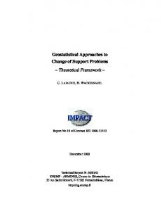
The study area is located in Bradford, a city in West Yorkshire, England. Bradford benefits from a maritime climate, with an average yearly rainfall of 873 mm recorded from 1981-2010 (MetOffice, UK). The rain gauge network, used in this study was located at the premises of Bradford University (Fig. 1) and rainfall data were collected from paired tipping bucket rain gauges placed at eight locations covering an area of 400 × 200 m2. Data used in this study was collected from April, 2012 to August, 20

2012 and from April, 2013 to August, 2013. These stations were located on selected roofs of the university buildings, thereby providing controlled, secure and obstruction-free measurement locations. Each station consists of two tipping bucket type rain gauges mounted 1m apart. On each roof the paired gauges were placed such that the height of the nearest obstruction is less than two times the distance between the gauges and the obstruction. An example of this design (Station 6) is also shown in Fig. 1. A histogram of the inter-station distances of the rain gauge network is presented in Fig. 2. Lag distances covered in this

25

network are distributed between 21 m (St. 4-St. 5) and 399 m (St. 1-St. 3). All rain gauges are ARG100 tipping bucket type with an orifice diameter of 254 mm and a resolution of 0.2 mm. Dynamic calibration was carried out for each individual gauge before deployment and visual checks were carried out every 4-5 weeks during the measurement period to make sure that the instruments were free of dirt and debris. Measurement (number of tips) were taken every minute and recorded on TinyTag data loggers mounted in each rain gauge. Quality control procedures were

30

performed prior to any statistical analysis, taking advantage of the paired gauge setup. The double-gauge design provides efficient quality control of the rain gauge data records as it helps to identify the instances when one of the gauges fails, and to flag the periods of missing or incorrect data (Ciach and Krajewski, 2006). During the dynamic calibration of all rain gauges it 3


was identified that there could be a maximum of ± 4 % difference in volume per tip between two rain gauges due to the tipping bucket mechanism. It was therefore decided that this is the maximum difference permitted between paired gauges. Hence every long set of cumulative data from paired gauges were checked against each other and if the difference were > ± 4 %, that complete set was identified as data affected by some type of measurement error (e.g. partial clogging caused by debris) and 5

they were removed from further analysis.

2.2

Characteristics of the data

The total average network rainfall depth for the summer seasons of 2012 and 2013 are 538 mm and 207 mm respectively. Figure 3 shows time series of daily rainfall averaged over the network for 2012 and 2103. There is a significant difference in cumulative rainfall between 2012 and 2013. The is because 2012 was the wettest year recorded in 100 years in UK (MetOffice, 10

UK) and 558 mm of rainfall during 2012 summer was unusually high. An average rainfall of only 360 mm was recorded during April to September over the 1981 - 2010 period at the nearest operational rain gauge station at Bingley, which is around 8 km from the study site with a similar ground elevation (MetOffice, UK). The data set for 2012 and 2013 contains 13 events yielding more than 10 mm network average rainfall depth and lasting for more than 20 min. A summary of these events is presented in Table 1. The total event duration ranges from 1.5 h to 11.4 h

15

while the event network average rainfall intensity varies from 1.79 mm/h to 7.96 mm/h. Table 1 also includes summary statistics of peaks of events (temporal averaging interval of 5 min) for the eight stations within the network. Although the spatial extent of the area is only 400 × 200 m2, it is clear that there is a considerable difference in rainfall intensity measurements indicated by the standard deviation and range of peaks observed in the individual events. The maximum standard deviation between peaks of individual events is 9.27 mm/h for event 8 which is around 12.5 % of the mean network peak

20

intensity of 74.4 mm/h. This shows the importance of analysing spatial uncertainty in the calculation of AARI even in such a small urban catchment. 3.

Methodology

Fig. 4 summarises the complete procedure of geostatistical upscaling of rainfall data adapted in this study in a step-by-step instruction followed by the detail description of each step. This complete procedure was repeated for temporal averaging 25

intervals of 2 min, 5 min, 15 min and 30 min to investigate the effect of temporal aggregation on prediction of AARI.

3.1

Step 1: Pooling of time steps

This rain gauge network contains eight measurement locations. These eight measurement locations give 28 spatial pairs at a given time instant which is far less than what geostatistics modelling requires. For example, (Webster and Oliver, 2007) recommends around 100 measurement points to calibrate a geostatistical model. The procedure adapted in this study increases 30

the number of pairs by pooling rainfall measurements for time instants with similar rainfall characteristics. With n measurement 4


locations and measurements taken at t time instants, the pooling over t time instants creates t × ½ × n × (n-1) spatial pairs. Although this procedure increases the number of spatial pairs by t times, the spatial lags for which information is available will be limited to the original configuration of the measurement locations, n. The underlying assumption of this pooling procedure is that the spatial variability over the pooled time instants is the same. 5

Therefore it is important to pool rainfall measurements with similar rainfall characteristics. Since the spatial rainfall variability is often intensity-dependent (Ciach and Krajewski, 2006), the characteristics of a less intense rainfall event may not be the same as that of a high intensity rainfall event. Hence to make the assumption of consistency of spatial variability, the range of rainfall intensity over the pooled time instants should be reasonably small. On the other hand, one should also make sure that there are enough time instants within a pooled subset to meet the data requirement to calibrate the geostatistical model. Based

10

on the above two criteria, three rainfall intensity classes were selected. The number of time instants (t) within each rainfall intensity class is presented for three temporal averaging intervals in Fig. 5. As expected, with increasing temporal averaging intervals the number of time instants t reduces. Figure 5 also shows that the higher the intensity, the smaller the t. There is a large difference between t for lower and higher intensity ranges which shows the dominance of lower intensity (0.1-5.0 mm/h) rainfall over the recording periods. For the 30 min temporal averaging interval there are only eight time instants for the

15

intensity range > 10 mm/h. This limits the maximum temporal averaging interval to 30 min for our analyses. But for a catchment of this size (400 × 200 m2) it is very unlikely to have a catchment response time of more than 30 min. Hence, from a

hydrological

point

of

view

consideration

of

temporal

averaging

intervals

longer

than

30 min would not be sensible.

3.2 20

Step 2: Standardisation of rainfall intensities

Having chosen the rainfall intensity classes to create pooled time instants, there can still be inconsistency in spatial variability between time instants within a class and therefore assuming a single geostatistical model for the whole subset may not be valid. To reduce this effect to a certain extent, all observations within an intensity class were standardised using mean and standard deviation of each and every time instant given by Eq. (1). Further steps were carried out on the standardised rainfall intensity. 𝑟𝑖𝑗 − 𝑚𝑖 𝑟̃𝑖𝑗 = (1) 𝑠𝑑𝑖

25

Where 𝑖=1… t where t is number of time instances; 𝑗=1… n where n is number of locations; 𝑟̃𝑖𝑗 is standardised rainfall intensity at a time step i and location j; 𝑟𝑖𝑗 is rainfall intensity at time step i and location j and; 𝑚𝑖 , 𝑠𝑑𝑖 are mean and standard deviation of rainfall intensities at time step i, respectively.

5


3.3

Step 3: Normal transformation of data

The upper part of Fig. 6 shows the distribution of standardised rainfall intensity for a temporal averaging interval of 5 min derived using Eq. (1). From the figure it is clear that the data do not follow a normal distribution. Distributions for other temporal averaging intervals (i.e. 2 min, 15 min and 30 min) show a similar behaviour. But the geostatistical upscaling method 5

to be used is based on the Gaussian distribution which means that it is assumed that the underlying data are from a normal distribution. This requires the rainfall data to be normally distributed prior to the calibration of the geostatistical model. Among the non-parametric transformation, Normal Score Transformation (NST, also known as normal quantile transformation (Van der Waerden, n.d.) is a widely used method to transform a variable distribution to the Gaussian distribution. It has widely been applied in many hydrological applications (Bogner et al., 2012; Montanari, A., & Brath, 2004; Todini, 2008; Weerts et al.,

10

2011). The concept of NST is to match the p-quantile of the data distribution of the p-quantile of the standard normal distribution. Consider a data variable z with cdf FZ (z). It will be transformed to a y-value with cdf FY (y) as follows 𝑦 = 𝐹𝑌−1 (𝐹𝑍 (𝑧))

(2)

Detailed description of NST including the steps involved can be found in number of studies including Bogner et al. (2012), Van der Waerden (1953) and Weerts et al. (2011). This method was applied to standardised rainfall intensity to make them 15

normally distributed. The lower part of Fig. 6 shows the transformed standardised intensity for the temporal averaging interval of 5 min.

3.4

Step 4: Calibration of Geostatistical model

A geostatistical model of rainfall intensity r (in our case normally transformed rainfall intensity derived from Section 3.3) at any location x can be written as: 20

𝑟(𝑥) = 𝑝(𝑥) + 𝜀(𝑥)

(3)

Where 𝑝(𝑥) is the trend (explanatory part) and 𝜀(𝑥) is the stochastic residual (unexplanatory part). Considering the availability of rainfall intensity data and scope of this study, it can be assumed that the trend is constant and does not depend on explanatory variables (e.g. topography of the area, wind direction). The stochastic term 𝜀 is spatially correlated and can be characterised by a variogram model. A variogram model typically consists of three parameters; nugget, sill and range (Isaaks and Srivastava, 25

1989). The nugget is the value of semi-variance at near-zero distance caused by measurement error and micro-scale spatial variation. It is negligibly small in the case of rainfall intensity data. The range is the distance beyond which the data are no longer spatially correlated. The sill is the maximum variogram value and equal to the variance of the variable of interest.

3.5

Step 5: Spatial stochastic simulation

During spatial interpolation, the assumption of a constant trend makes this an ordinary kriging system (Isaaks and Srivastava, 30

1989) which is given by the following set of equations 6


𝑞

∑ 𝑤𝑘 𝛾𝑙𝑘 − 𝜇 = 𝛾𝑙0

∀ 𝑙 = 1, … , 𝑞

(4)

𝑘=1 𝑞

∑ 𝑤𝑙 = 1

(5)

𝑙=1

Where 𝑙, 𝑘 are indices; the 𝑤𝑙 , 𝑙 = 1, … , 𝑞 are ordinary kriging weights; 𝛾𝑙𝑘 is the semivariance between rainfall intensities at 5

locations𝑥𝑙 and 𝑥𝑘 ; 𝛾𝑙0 is the semivariance between rainfall intensities at location 𝑥𝑙 and prediction location𝑥0 , and 𝜇 is a Lagrange parameter. Once the ordinary kriging weights, which give the minimum prediction error variance, are calculated using Eq. (4) and Eq. (5), point rainfall intensities can be calculated using point kriging at any given point. But we need a change of support from point to block as our intention is to estimate the rainfall intensity over the catchment. This is usually done by simply predicting at all points inside the catchment and then integrating over the catchment (this procedure is known

10

as block kriging). But the procedure of NST as explained in Section 3.4 also involves back-transformation of kriging predictions to the original domain at the end (Step 6). Since this transformation is typically non-linear, the back-transform of the spatial average of the transformed variable that is obtained from block kriging is not the same as the spatial average of the back-transformed variable; we need the latter and not the former. Hence block kriging cannot be applied. The alternative used in this study is to use a computationally more demanding spatial stochastic simulation which involves generation of a larger

15

number of possible realisations and spatial aggregation of these realisations. Unlike kriging spatial stochastic simulation do not aim to minimizing a local error variance but focus on the reproduction of the statistics such as the histogram or semivariogram model (Goovaerts, 2000). The output from spatial stochastic realisation is a set of alternative realisations of rainfall predictions at user defined grid points. The differences among these realisations are used as a measure of uncertainty. In this study, a grid with cells of 25 m × 25 m was laid over the study area and 500 simulations of transformed rainfall at grid

20

cell centres were generated using spatial stochastic simulation for each time step. This grid size and number of simulations were selected considering the spatial resolution of available measurements and computational demand. It was observed that neither finer grid nor more simulation improves the predictions much.

3.6

Step 6-9: Calculation of AARI and associated uncertainty

Once we derived all realisations from the spatial stochastic simulation the next step is to transform them to the original domain 25

using back-transformation (NST-1). Some values derived from spatial stochastic simulation were outside the transformed data range. Hence during back transformation (step 6) of these values linear extrapolation was used. These linear models were derived using a selected number of head and tail portion of normal Q-Q plot. This is one of the simplest and most commonly used solutions for NST back-transformation (Bogner et al., 2012; Weerts et al., 2011). Considering the scope of this study and the relatively small number of data which had to be extrapolated, other extrapolation methods have not been explored. 7


Having transformed all realisations to the original domain the next step is spatial aggregation (step 7) of each and every simulation which gives us m (=500) simulations of the areal mean. The mean prediction (𝑝̅) and standard deviation (𝑠𝑝 ) were then calculated using Eq. (6) and Eq. (7) respectively (Step 8). 𝑚

5

𝑝̅ = ∑ 𝑝𝑥

(6)

𝑖=1 𝑚

1 𝑠𝑝 = √ ∑(𝑝𝑖 − 𝑝̅ ) 𝑚

(7)

𝑖=1

Where px is prediction from the i-th simulation. Finally, by doing the inverse standardisation of 𝑝̅ and 𝑠𝑝 to account for step 2, the AARI and associated uncertainty measure (standard deviation) were derived (Step 9). 10

4.

4.1

Results and Discussion

Calibration of the geostatistical model of rainfall

As explained in Section 3.4, the geostatistical model of transformed rainfall data was calibrated using variograms for three different intensity ranges. This procedure was repeated for temporal averaging intervals of 2 min, 5 min, 15 min and 30 min. Exponential models were fitted to empirical semi variograms. The resulting variograms are presented in Fig. 7. 15

The variograms illustrate two properties of the collected rainfall measurements; spatial variability of rainfall, and measurement error. Theoretically at zero lag distance the variance should be zero. However most of these variograms exhibit a positive nugget effect (generally presented as nugget-to-sill ratio) at zero lag distance due to measurement error. From Fig. 7 it is clear that the nugget-to-sill ratio varies with both rainfall intensity class and temporal averaging interval. Considering the behaviour of nugget-to-still ratio against rainfall intensity class, it can be observed that the smaller the intensity

20

the higher the nugget-to-sill ratio, regardless of temporal averaging interval. For example, at 2 min averaging interval the nugget-to-still ratio increases from zero to almost one (nugget variogram) as rainfall intensity class changes from > 10 mm/h to < 5 mm/h. Looking at the behaviour of nugget-to-still ratio against temporal averaging interval, Fig. 7 shows that the smaller the averaging interval the higher the nugget-to-still ratio, regardless of rainfall intensity class. For example for rainfall intensity class of 5.0–10.0 mm/h the nugget-to-still ratio decrease from almost one to zero as the temporal averaging interval increases

25

from 2 min to 30 min. These observations show that the measurement error characterised by nugget-to-still ratio (a) decreases with increasing rainfall intensity class and (b) decreases with increasing averaging interval. This behaviour of measurement error against rainfall intensity and averaging interval is mainly attributed to measurementrelated error of tipping bucket type rain gauges (hereafter referred as TB error). This is due to the rain gauges’ inability to 8


capture small temporal variability of the rainfall time series. The behaviour of TB error against rainfall intensity and temporal averaging interval as seen from Fig. 7 complements results from previous studies (Habib et al., 2001; Villarini et al., 2008). Habib et al. (2001) in their study found similar behaviour of TB error with increasing averaging interval (1 min, 5 min and 15 min) and also with increasing intensity (0-100 mm/h). Although the bucket size used in their study (0.254 mm) is slightly 5

different from our rain gauge bucket size of 0.2 mm, the characteristic of the TB error against rainfall intensity for different averaging interval is consistent in both cases. It is clear from Fig. 7 that the spatial correlation of rainfall intensity improves with increasing temporal averaging interval. Decorrelation distance (range) is a good indicator of the improvement in spatial correlation. At lower temporal averaging intervals (≤ 5 min) the variograms for all rainfall intensity classes reach the decorrelation distance very quickly (< 100 m). But

10

at averaging intervals ≥ 15 min, the decorrelation distance has not been reached even at a maximum separation distance, showing the improvement in spatial correlation. High spatial variability of rainfall at shorter temporal averaging interval (≤ 5 min) is an important observation in the context of urban drainage run off modelling, as the time step used in such models is generally around 2 min for small catchments. The increase in spatial correlation of rainfall intensity with increasing temporal averaging interval is an expected observation and agree with other similar studies (Ciach and Krajewski, 2006; Krajewski et

15

al., 2003; Villarini et al., 2008). For example, Krajewski et al. (2003) in their study on analysis of spatial correlation structure in small-scale rainfall in central Oklahoma observed similar behaviour using correlogram functions for different temporal averaging intervals. The behaviour of spatial correlation against rainfall intensity class is not very distinctive from Fig. 7. At lower temporal averaging intervals (≤ 5 min) the variograms for different rainfall intensity classes look similar apart from the nugget effect

20

caused by TB error. At averaging intervals ≥ 15 min, variograms for rainfall intensity classes 5.0–10.0 mm/h and > 10 mm/h looks similar, showing a common pattern of spatial correlation.

4.2

Geostatistical upscaling of rainfall data

Having calculated all variograms, the next step is to apply spatial stochastic simulation for the time instants of interest followed by steps 6 to 9 in Fig. 4 to calculate the AARI together with associated uncertainty. This procedure was carried out for all 25

events presented in Table 1. The following sections present and discuss the predicted AARI and associated uncertainty levels derived from step 9. 4.2.1

Prediction error vs AARI

The scatter plot in Fig. 8 shows the prediction standard deviation plotted against predicted AARI at 5 min averaging interval for all time instants of all events presented in Table 1. The uncertainty level represented by the standard deviation is due to the 30

combined effect of both spatial variability of rainfall and TB error in the rainfall data. Most of the time the coefficient of

9


variation (CV, refer Eq. (8)) is around 5 % which is not high. But there are also instances where it is more than 10 % with a maximum of 13 % corresponding to a predicted rainfall of 11 mm/h. 𝐶𝑉 =

𝐴𝐴𝑅𝐼 𝑝𝑟𝑒𝑑𝑖𝑐𝑡𝑖𝑜𝑛 𝑒𝑟𝑟𝑜𝑟 𝑠𝑡𝑎𝑛𝑑𝑎𝑟𝑑 𝑑𝑒𝑣𝑖𝑎𝑡𝑖𝑜𝑛 𝑃𝑟𝑒𝑑𝑖𝑐𝑡𝑒𝑑 𝐴𝐴𝑅𝐼

(8)

As expected, a large portion of the predicted AARI is within 0-10 mm/h. The corresponding standard deviations are highly 5

scattered, possibly due to the large TB error for rainfall intensities smaller than 10 mm/h as already seen from Fig. 7, where the nugget-to-still ratio is close to one at this intensity range. In this range there are also a few small clusters of points separated from the larger cluster with almost zero standard deviation, even for a predicted AARI of around 8 mm/h. It shows a consistent rainfall over the area at these time instants which results in a very small standard deviation in the predicted AARI. 4.2.2

10

Prediction error vs temporal averaging interval

Having analysed the behaviour of the prediction error against predicted AARI, this section presents the effect of temporal averaging interval on the prediction error of AARI. Figure 9 shows the kriging predictions with 95 % prediction intervals derived from the prediction standard deviation for temporal averaging intervals of 2 min, 5 min, 15 min and 30 min for event 11. Event 11 represent average conditions roughly in terms of event duration and peak intensity. Prediction errors of other events against the temporal averaging interval follow the same pattern of behaviour.

15

It is expected that with increasing temporal averaging interval the local minima and maxima of AARI get smoothed out. Here it can be noted that in this event this effect decreases the event peak AARI from around 50 mm/h to around 20 mm/h as the temporal averaging interval increases from 2 min to 30 min. It shows the importance of selecting appropriate temporal scales in the hydrologic modelling of small urban catchments (10-20 ha) where the time steps will be in the range of 2 to 5 min. But on the other hand the larger the temporal averaging interval, the smaller the prediction interval and the smaller the level of

20

uncertainty. The reason is that with increasing temporal averaging interval while the spatial correlation of rainfall improves the TB error becomes smaller as seen from the variogram in Fig. 7. In fact when the averaging interval is larger than 15 min the prediction interval width becomes negligible. But as mentioned above, temporal scales of interest in urban hydrology of similar sized catchment can be as small as 2 min where there is still considerable uncertainty. The 95 % prediction interval shows around ± 13 % of error in rainfall intensity corresponding to a prediction of peak rainfall of 47 mm/h at 2 min averaging

25

interval. The decreasing trend of uncertainty in the prediction of AARI with increasing temporal averaging interval agrees with a previous study by Villarini et al. (2008). Although the spatial extend of their study is much larger (360 km2), their results also show that the spatial sampling uncertainties tend to decrease with increasing temporal averaging interval due to improvement in measurement accuracy and increased spatial correlation.

30

4.2.3

Prediction of peak rainfall intensity

Rainfall event peaks are of significant interest in urban hydrology as most of the hydraulic structures in urban drainage systems are designed based on peak discharge which is often derived from peak rainfall. Hence it is important to consider the 10


uncertainty in prediction of peaks of AARI. Figure 10 presents predicted peaks of AARI for all 13 events presented in Table 1, together with corresponding 95 % prediction intervals indicated by vertical bars. The peak intensities range from 6 mm/h to 92 mm/h at 2 min averaging interval and this range narrows down to 3 mm/h – 21 mm/h at averaging interval of 30 min. In general, Fig. 10 shows that (a) the larger the peak value the larger the prediction interval and (b) the larger the temporal 5

averaging interval the smaller the prediction interval. Another interesting observation is that the prediction intervals for smaller peaks (< 20 mm/h) are very small even at an averaging interval of 2 min, where both spatial variability and TB error are at their maximum. But it should be noted that the prediction interval in Fig. 9 and Fig. 10 are derived from standard deviation, a measure which is proportional to the mean. Hence it is important to look at the CV, a normalised measure, (refer Eq. (8)) of these predictions together with their prediction

10

interval to get a clearer picture of uncertainty. 4.2.4

Prediction vs CV

CV against all predicted peaks of AARI are presented in Fig. 11. This plot is divided in two segments based on predicted AARI at a threshold value of 10 mm/h to analyse the effect of lower and higher rainfall intensity on CV. Regardless of the range of intensity, CV decreases with averaging interval which is what we expected. Considering CV against intensity range, in general 15

CV is higher when the predicted intensity is lower than 10 mm/h for all temporal averaging intervals. It compliments what is observed from the variograms in Fig. 7, where below 10 mm/h the TB error becomes high. Hence it is expected to see a higher uncertainty characterised by CV at lower rainfall intensity (< 10 mm/h) especially at a temporal averaging interval of 2 min where the TB error is at its highest. But when the temporal averaging interval is 30 min where the TB error is at its lowest, the difference between CV for lower (< 10 mm/h) and higher (> 10 mm/h) intensity becomes smaller. At 30 min averaging interval

20

the mean CV below and above 10 mm/h are 1.7 % and 1.2 % respectively, but they increase to 6.6 % and 3.5 % at 2 min averaging interval. The maximum CV at 2 min averaging interval are 13 % and 6.8 % for lower (< 10 mm/h) and higher (> 10 mm/h) rainfall intensity respectively. This is fairly high considering the required accuracy defined in standard guidelines of urban hydrological modelling practises. For example urban drainage verification guidelines (WaPUG, 2012) in UK set a maximum allowable deviation of 25 % to -15 % in peak runoff demanding more accurate prediction of rainfall which is the

25

main driver of the runoff process. Hence a better trade-off between temporal resolution and accuracy in catchment rainfall prediction is needed when deciding the time step of hydrologic modelling of small urban catchments. 5.

Conclusions

In this study we presented a method to predict AARI together with associated uncertainty using geostatistical upscaling. Rainfall data collected from a cluster of eight paired rain gauges in a 400 × 200 m2 urban catchment in Bradford, UK were 30

used in this study. We quantified the level of uncertainty in the prediction of AARI for different combinations of temporal averaging intervals, ranging from 2 to 30 min, and rainfall intensity ranges.

11


A summary of the significant findings are listed below, 

The level of uncertainty in the prediction of AARI using point measurement data essentially comes from two sources; spatial variability of the rainfall and TB error. The significance and characteristics of the TB error observed here corresponds to sampling related error of tipping bucket type rain gauges and may vary for other types of rain

5

gauges. 

At smaller temporal averaging intervals, the effect of both spatial variability and TB error is high, resulting in higher uncertainty levels in the prediction of AARI especially for lower intensity rain (at 2 min temporal averaging interval the average CV is 6.6 % and the maximum CV is 13 %). With increasing temporal averaging interval the uncertainty becomes lower as the spatial correlation improves and the TB error reduces (at 30 min averaging interval the average

10

CV is 1-2 %). 

With increasing temporal averaging interval while the uncertainty decreases, the predicted peaks of AARI reduces significantly (e.g. peak of event 8 reducing to 21 mm/h from 92 mm/h when averaging interval increases from 2 min to 30 min). Hence a careful trade-off between temporal resolution and accuracy in rainfall prediction is needed to decide the most appropriate time step for averaging point rainfall data for urban hydrologic applications.

15



TB error at averaging intervals of less than 5 min, especially at low intensity rainfall measurements, is as significant as spatial variability. Hence proper attention to TB error should be given in any application of these measurements, especially in urban hydrology where averaging interval are often as small as 2 min.

Although spatial stochastic simulation used in this study needs more computational power than block kriging, it is a robust approach and allows data transformation during spatial interpolation. Such data transformation is important to ensure that 20

rainfall data satisfy the normality assumption of ordinary kriging. The pooling procedure used in this study makes use of the continuous measurement of rainfall and helps provide a solution to meet the data requirements for geostatistical interpolation methods to a certain extent. An urban catchment of this size needs rainfall data at a temporal and spatial resolution which current radar data technology cannot meet. In addition the level of uncertainty in radar measurements would be much higher than that of point measurements

25

especially at a fine averaging interval (< 5 min) which are often of interest in urban hydrology. Hence experimental rain gauge data similar to the one used in this study are crucial for similar studies focused on small urban catchments. Furthermore, the paired gauges setup used in rainfall data collection improves the reliability on rainfall data as it helps to flag the missing or wrong dataset of the measurements and it consequently helps efficient quality control of the data. Results from this study can be used for uncertainty analyses of hydrologic and hydrodynamic modelling of similar sized urban

30

catchments as it provides information on uncertainty associated with rainfall estimation which is arguably the most important input in these models. This will help to differentiate input uncertainty from total uncertainty thereby helping to understand other sources of uncertainty due to model parameter and model structure. This information can help to avoid false calibration and force fitting of model parameters (Vrugt et al., 2008). This study can also help to judge optimal temporal averaging interval for rainfall estimation of hydrologic and hydrodynamic modelling especially for small urban catchments. 12


Acknowledgements This research work is done as a part of Marie Curie ITN - Quantifying Uncertainty in Integrated Catchment Studies (QUICS). This project has received funding from the European Union’s Seventh Framework Programme for research, technological development and demonstration under grant agreement no 607000. 5

13


References Berne, A., Delrieu, G., Creutin, J. D. and Obled, C.: Temporal and spatial resolution of rainfall measurements required for urban hydrology, J. Hydrol., 299(3-4), 166–179, doi:10.1016/j.jhydrol.2004.08.002, 2004. Bogner, K., Pappenberger, F. and Cloke, H. L.: Technical Note: The normal quantile transformation and its application in a 5

flood forecasting system, Hydrol. Earth Syst. Sci., 16(4), 1085–1094, doi:10.5194/hess-16-1085-2012, 2012. Chow, V. Te: Handbook of Applied Hydrology. A compendium of water-resources technology, McGraw-Hill, New York., 1964. Ciach, G. J. and Krajewski, W. F.: Analysis and modeling of spatial correlation structure in small-scale rainfall in Central Oklahoma, Adv. Water Resour., 29, 1450–1463, doi:10.1016/j.advwatres.2005.11.003, 2006.

10

Dirks, K. N., Hay, J. E., Stow, C. D. and Harris, D.: High-resolution studies of rainfall on Norfolk Island Part II: Interpolation of rainfall data, J. Hydrol., 208(3-4), 187–193, doi:10.1016/S0022-1694(98)00155-3, 1998. Emmanuel, I., Andrieu, H., Leblois, E. and Flahaut, B.: Temporal and spatial variability of rainfall at the urban hydrological scale, J. Hydrol., 430-431, 162–172, doi:10.1016/j.jhydrol.2012.02.013, 2012. Gires, A., Onof, C., Maksimovic, C., Schertzer, D., Tchiguirinskaia, I. and Simoes, N.: Quantifying the impact of small scale

15

unmeasured rainfall variability on urban runoff through multifractal downscaling: A case study, J. Hydrol., 442-443, 117– 128, doi:10.1016/j.jhydrol.2012.04.005, 2012. Gires, A., Tchiguirinskaia, I., Schertzer, D., Schellart, A., Berne, A. and Lovejoy, S.: Influence of small scale rainfall variability on

standard

comparison

tools

between

radar

and

rain

gauge

data,

Atmos.

Res.,

138,

125–138,

doi:10.1016/j.atmosres.2013.11.008, 2014. 20

Glasbey, C. A. and Nevison, I. M.: Modelling Longitudinal and Spatially Correlated Data, edited by T. G. Gregoire, D. R. Brillinger, P. J. Diggle, E. Russek-Cohen, W. G. Warren, and R. D. Wolfinger, pp. 233–242, Springer New York, New York, NY., 1997. Goovaerts, P.: Estimation or simulation of soil properties? An optimization problem with conflicting criteria, Geoderma, 97(34), 165–186, doi:10.1016/S0016-7061(00)00037-9, 2000.

25

Habib, E., Krajewski, W. F. and Kruger, A.: Sampling Errors of Tipping-Bucket Rain Gauge Measurements, J. Hydrol. Eng., 6(2), 159–166, doi:10.1061/(ASCE)1084-0699(2001)6:2(159), 2001. Isaaks, E. H. and Srivastava, R. M.: An Introduction to Applied Geostatistics, Oxford University Press, New York, USA., 1989. Jaffrain, J. and Berne, A.: Quantification of the small-scale spatial structure of the raindrop size distribution from a network

30

of disdrometers, J. Appl. Meteorol. Climatol., 51(5), 941–953, doi:10.1175/JAMC-D-11-0136.1, 2012. Krajewski, W. F., Ciach, G. J. and Habib, E.: An analysis of small-scale rainfall variability in different climatic regimes, Hydrol. Sci. J., 48(2), 151–162, doi:10.1623/hysj.48.2.151.44694, 2003. Lloyd, C. D.: Assessing the effect of integrating elevation data into the estimation of monthly precipitation in Great Britain, J.

14


Hydrol., 308(1-4), 128–150, doi:10.1016/j.jhydrol.2004.10.026, 2005. Ly, S., Charles, C. and Degré, A.: Different methods for spatial interpolation of rainfall data for operational hydrology and hydrological modeling at watershed scale : a review, Biotechnol. Agron. Soc. Environ., 17(2), 392–406, 2013. Mair, A. and Fares, A.: Comparison of Rainfall Interpolation Methods in a Mountainous Region of a Tropical Island, , (April), 5

doi:10.1061/(ASCE)HE.1943-5584.0000330., 2011. MetOffice UK: MetOffice, UK, [online] Available from: http://www.metoffice.gov.uk/ (Accessed 25 November 2015), n.d. Montanari, A., & Brath, A.: A stochastic approach for assessing the uncertainty of rainfall-runoff simulations, Water Resour. Res., 40(1), 1–11, doi:10.1029/2003WR002540, 2004. Nalder, I. a. and Wein, R. W.: Spatial interpolation of climatic Normals: test of a new method in the Canadian boreal forest,

10

Agric. For. Meteorol., 92, 211–225, doi:10.1016/S0168-1923(98)00102-6, 1998. Ochoa-Rodriguez, S., Wang, L. P., Gires, A., Pina, R. D., Reinoso-Rondinel, R., Bruni, G., Ichiba, A., Gaitan, S., Cristiano, E., van Assel, J., Kroll, S., Murlà-Tuyls, D., Tisserand, B., Schertzer, D., Tchiguirinskaia, I., Onof, C., Willems, P. and ten Veldhuis, M. C.: Impact of spatial and temporal resolution of rainfall inputs on urban hydrodynamic modelling outputs: A multi-catchment investigation, J. Hydrol., 531, 389–407, doi:10.1016/j.jhydrol.2015.05.035, 2015.

15

Schuurmans, J. M. and Bierkens, M. F. P.: Effect of spatial distribution of daily rainfall on interior catchment response of a distributed hydrological model, Hydrol. Earth Syst. Sci., 3(4), 2175–2208, doi:10.5194/hessd-3-2175-2006, 2006. Tabios III, G. Q. and Salas, J. D.: A comparative analysis of techniques for spatial interpolation of precipitation, J. Am. Water Resour. Assoc., 21(3), 365–380, 1985. Todini, E.: A model conditional processor to assess predictive uncertainty in flood forecasting, Int. J. River Basin Manag.,

20

6(2), 123–137, doi:10.1080/15715124.2008.9635342, 2008. Villarini, G., Mandapaka, P. V., Krajewski, W. F. and Moore, R. J.: Rainfall and sampling uncertainties: A rain gauge perspective, J. Geophys. Res. Atmos., 113(11), 1–12, doi:10.1029/2007JD009214, 2008. Vrugt, J. a., ter Braak, C. J. F., Clark, M. P., Hyman, J. M. and Robinson, B. a.: Treatment of input uncertainty in hydrologic modeling: Doing hydrology backward with Markov chain Monte Carlo simulation, Water Resour. Res., 44(12),

25

doi:10.1029/2007WR006720, 2008. Van der Waerden, B. L. .: Order tests for two-sample problem and their power I-III, Indag. Math., 14,15, 453–458 (14), 303– 316(15), n.d. Webster, R. and Oliver, M. a: Geostatistics for environmental scientists, Second edi., John Wiley & Sons, Ltd, West Sussex, England., 2007.

30

Weerts, A. H., Winsemius, H. C. and Verkade, J. S.: Estimation of predictive hydrological uncertainty using quantile regression: examples from the National Flood Forecasting System (England and Wales), Hydrol. Earth Syst. Sci., 15(1), 255–265, doi:10.5194/hess-15-255-2011, 2011.

15


Table 1: Summary of events which yielded more than 10 mm rainfall and lasted for more than 20 min with summary statistics of event peaks (derived at 5 min temporal averaging interval) from all stations.

Event ID.

Date

Network

Network

Network

Summary statistics of peaks

average

average

average

between different stations (mm/h)

duration (h)

intensity (mm/h)

rainfall (mm)

Mean

Std. Dev

Max

Min

1

18/04/2012

6.33

2.20

13.9

5.10

0.550

6.02

4.74

2

25/04/2012

6.42

2.55

16.3

7.05

0.751

8.32

5.92

3

09/05/2012

8.92

1.79

16.0

5.10

0.537

5.97

4.74

4

14/06/2012

6.83

1.99

13.6

5.25

0.636

6.04

4.74

5

22/06/2012

11.4

2.39

27.3

12.7

1.72

15.4

9.67

6

06/07/2012

4.42

5.31

23.4

38.5

4.52

42.9

30.5

7

06/07/2012

3.25

3.23

10.5

7.20

0.679

8.46

5.93

8

07/07/2012

1.50

7.84

11.8

74.4

9.27

86.5

61.9

9

19/07/2012

3.08

3.35

10.3

12.7

2.01

14.5

9.74

10

15/08/2012

2.00

7.96

15.9

43.0

3.69

47.8

37.5

11

14/05/2013

7.92

2.14

17.0

8.08

1.20

9.55

6.09

12

23/07/2013

1.75

6.51

11.4

37.7

2.09

42.6

35.7

13

27/07/2013

8.17

4.34

35.5

26.6

1.23

27.5

23.8

5

10

16


5

10 200 m × 400 m

Figure 1: (Left) A aerial view of - rain gauge network covering an area of 200 × 400 m2 at Bradford University, UK. (Right) A photograph of paired rain gauges at station 6.

15

20

25

17


Frequency [-]

12 9 6 3 0 100

200

300

400

Inter station distance [m] Figure 2: Histogram with class interval width of 100 m showing frequency distribution of inter-station distances (m)

5

10

15

20

18


5

10

Figure 3 : Time series of network average daily rainfall in the two seasons of 2012 and 2013 with vertical dashed lines indicating the events presented in Table 1

15

20

19


1. Pooling of time steps using predefined range of rainfall intensities, R

2. Standardisation of rainfall intensities, 𝑅= S(R) 5

3. Normal quantile transformation of standardised intensities, 𝑅 N = NST(𝑅) 10 4. Calibration of Geostatistical model for 𝑅 N in the form of variogram

5. Spatial stochastic simulation using a large number of possible realisations 15

of 𝑅 N

6. Back transformation of all realisation using NST-1

20

7. Spatial aggregation of each of the back transformed simulations

8. Estimation of the mean prediction (mean of the aggregates) and standard deviation (standard deviation of the aggregates)

25

9. Inverse standardisation of mean prediction (=AARI) and standard deviation (uncertainty measure) using S-1 Figure 4: Step by step procedure developed in this study to predict AARI and associated level of uncertainty. Boxes highlighted in dots indicate the steps to resolve the problem of scarcity in measurement locations, grey boxes show the steps introduced to address non-normality of rainfall data.

20


Number of samples

100000 10000 1000 100 10 1 2

5

15

30

Temporal averaging interval (min) < 5.0 mm/hr

5.0-10.0 mm/hr

>10.0 mm/hr

Figure 5 : Number of time instants for each temporal averaging interval and rainfall intensity class combination

21


5

NST

10

15

20

Figure 6: Distribution of standardised rainfall intensity for different rainfall intensity classes at a temporal averaging interval of 5 min before (upper part) and after (lower part) normal score transformation (NST)

22


Figure 7: Calculated variograms for each temporal averaging interval and for each range of intensity within a temporal averaging interval

23


Figure 8: AARI standard deviation (prediction error) against predicted AARI for averaging interval of 5 min

24


Figure 9 : Predictions of AARI (indicated by points) together with 95 % prediction intervals (indicated by grey ribbon) for rainfall event 11 for different averaging intervals

25


Figure 10 : Predictions of event peaks of AARI (indicated by points) and 95 % prediction intervals (indicated by vertical bars) for the events presented in Table 1

26


Figure 11: Coefficient of variation plotted against predicted peaks of AARI for the events presented in Table 1

27

Geostatistical upscaling of rain gauge data to support uncertainty ...

Geostatistical upscaling of rain gauge data to support uncertainty ...

Suggest Documents