Abstract. The distribution of submerged macrophytes in the littoral zone of Lake Geneva (Switzerland) was modeled from bathymetry, wave exposure, current ...
Plant Ecology 139: 113–124, 1998. © 1998 Kluwer Academic Publishers. Printed in the Netherlands.
113
GIS modeling of submerged macrophyte distribution using Generalized Additive Models Anthony Lehmann Laboratoire d’Ecologie et de Biologie Aquatique, Facult´e des Sciences, Universit´e de Gen`eve, 18 ch. des Clochettes, 1206 Geneva, Switzerland Received 3 November 1997; accepted in revised form 20 July 1998
Key words: Aquatic macrophyte, GIS habitat modeling, Gradient analysis, Generalized Additive Models, Potamogeton, Characea
Abstract The distribution of submerged macrophytes in the littoral zone of Lake Geneva (Switzerland) was modeled from bathymetry, wave exposure, current strength, water quality, soil type and harvesting practice. Generalized Additive Models (GAM) were used to identify the responses of three Potamogeton species and Chara sp. to these environmental parameters. The maps of original data and the spatial predictions were processed in a Geographic Information System (GIS) database. The effect of the selected environmental variables on plant distribution is discussed in relation to species adaptive strategies. GIS and GAM appear as powerful tools to proceed from the description of species response curves to environmental gradients toward the spatial predictions of species distribution under changing environmental conditions.
Introduction Many theories have been proposed to explain and predict terrestrial vegetation distribution along environmental gradients, especially in relation to interspecific competition (see Grace & Tilman 1990). Several authors have attempted to adapt these models to the specific environmental conditions found in aquatic ecosystems such as lake littorals. In a review of sediment interactions with submerged macrophytes, Barko et al. (1991) suggested that Tilman’s (1982) concept of resource partitioning as a result of plant competition is a valuable hypothesis to test with aquatic vegetation along sediment resource gradients. This theory had been tested and rejected earlier by Anderson & Kalff (1986) in a uniform bed of submerged vegetation. These authors suggested that Grime’s C-S-R model (Grime 1979; Grime et al. 1988) was more appropriate to explain observed patterns of distribution. Kautsky (1988) effectively evaluated the C-S-R model for submerged aquatic macrophytes. In order to take into account the differences in life strategies
found in aquatic environments, she proposed to split the stress-tolerant strategy into ‘stunted’ and ‘biomass storer’ species. In a recent study, Lehmann et al. (1997a, b) also used Grime’s theory to explain the distribution of three different species of Potamogeton but failed to predict their distribution. In wetland plant communities, Keddy (1990, 1992), and Wisheu & Keddy (1992) described patterns of species pool, diversity and life forms along productivity and disturbance gradients through the definition of a new process-oriented model: the centrifugal organization. This model defines a core habitat, which is preferred by all species, and a series of peripheral habitats in which different specialized species occur. In order to predict the distribution of communities, Keddy proposed a set of two methods called ‘assembly rules’ and ‘response rules’. The former predicts which subset of a species pool will tolerate given environmental conditions and form an observed community. The latter specifies how an initial pool of species will respond to environmental changes. Assembly rules and response rules are based on the knowledge of mor-
114 phological, physiological and ecological traits of each species. Austin (1990; Austin & Smith 1989; Austin & Gaywood 1994) presented another model based on the continuum concept (Gauch & Whittaker 1972) which is not process-oriented as Tilman’s, Grime’s or Keddy’s theories and has not yet been tested on aquatic vegetation. In their search for predictive models, Austin et al. (1984, 1990, 1994) have taken advantages of modern statistical analyses such as Generalized Linear Models (GLM). GLM present several advantages over classical multiple regressions: they accommodate data from different statistical distributions with appropriate statistical error modeling (e.g., normal binomial, ordinal, Poisson or negative binomial). This more general formulation of regression models also allows combining continuous variables (e.g., depth) and categorical variables (e.g., substrate type). A non-parametric extension of GLM, Generalized Additive Models (GAM), has also been used in vegetation studies (e.g., Yee & Mitchell 1991; Leathwick 1995). GAMs build a model using smoothed functions derived from the explanatory variables, instead of pre-establishing a parametric model. This allows testing whether a response curve is bell-shaped or not, and to compare directly the additive effect of each explanatory variable from its response curves in the prediction. While GLM have already been used in combination with Geographic Information Systems (GIS) to produce spatial predictions of vegetation distribution (e.g., van de Rijt et al. 1996; Guisan et al. 1998), the non-parametric nature of GAM represent an obstacle to the combining of maps of environmental variables in standard GIS overlay. In aquatic vegetation studies, GIS have been used in numerous applications (see Lachavanne et al. 1997). GIS modeling of aquatic plant distribution was performed using simple Boolean logic (Jensen et al. 1992) and logistic multiple regression (Narumalani et al. 1997). These two studies focused on emergent and floating vegetation using the following explanatory variables: water depth, slope, exposure to wave action (fetch) and substrate type. The aim of this study is to show how GAM and GIS can be combined to predict vegetation distribution as advocated by most current theories and as needed in applied perspectives. The proposed methodology is used to predict the distribution of three submerged macrophyte species (Potamogeton pectinatus L., P. lucens L., P. perfoliatus L.) and one
taxa Chara sp. (composed here of Chara contraria A.Br., Chara globularis Thuillier and Nitellopsis obtusa J.Gr.). Species distribution is modeled from presence-absence data combined with four continuous environmental variables: water depth, fetch, current strength, water quality, and two categorical environmental variables: substrate type and harvesting practice. These models are also used to predict distribution under hypothetical changes of environmental variables such as water quality and water level.
GIS database development Vegetation Submerged vegetation was mapped from 28 aerial photographs (∼1:5000) and field surveys in July 1995. The cartographic methodology is described in detail in Lehmann & Lachavanne (submitted). Vegetated areas appear generally darker than bare substrate and can therefore be semi-automatically separated on scanned aerial photographs (Lehmann et al. 1997b). Areas colonized by filamentous algae were distinguished from macrophytes during field survey. These photographs and the extracted vegetation zones were georeferenced from six shore and two offshore control points using ILWIS software (International Institute for Aerospace Survey and Earth Sciences, The Netherlands). The 28 vegetation maps were joined in a single map in ARCVIEW software (Environmental Systems Research Institute, California). Basic attributes for each field observed vegetation zone were surface area, cover index and species composition. Derived attributes were calculated: abundance index (Lachavanne et al. 1985), nutrient load index (Melzer 1988) and saprobity index (Husak et al. 1989) (see Lehmann & Lachavanne, submitted). For this study, maps of presence-absence of four taxa (Potamogeton pectinatus L., Potamogeton lucens L., Potamogeton perfoliatus L. and Chara sp.) were derived. Bathymetry Bathymetry was mapped in 1997 from an echosounding survey consisting of 250 transects perpendicular to the shore (1–15 m depth range), and separated by a maximum distance of 100 m. This information was recorded on an echosounder (Bathy 1000, Ocean Data Equipment Corporation, MA) combined to differential GPS positions (GPS45, Garmin, Kansas), with a
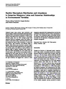
115 10 m horizontal precision. A total of 50 000 georeferenced depth points were extracted from these files and spatially interpolated in SURFER (Golden Software, Colorado) using a simple linear Kriging method. The resulting map was rasterized to a spatial resolution of 5 m in ARCVIEW Spatial Analyst extension with a vertical precision estimated to be 25cm (Figure 1a). Effective fetch Fetch is a distance on open water in a given angular direction. It was calculated in ARCVIEW with a script (available on request from the author) on 3300 points (50 m grid base), every 6◦ from the North . Effective fetch gives a more representative measure of how the wind governs the waves (length and height) since it is a weighted distance of fetch around a wind direction (±42◦) (Håkanson 1981). It was calculated with the direction of the two dominant winds in the area (La Bise 42◦ and Le Vent 220◦). The higher effective fetch of either wind direction was calculated and rasterized to the same resolution of the bathymetric map (5 m) (Figure 1b). Current strength As the study area is close to the outlet of Lake Geneva (the Rhône river), its complex current dynamic was globally estimated by the distance from the outgoing river. As water currents are normally exponentially related to the distance from the output, values were transformed accordingly. This method remains certainly very approximate in the absence of field measured data, but it is used here as a proxy for actual current impact on macrophytes (Figure 1c). Water pollution Water pollution along the littoral zone was measured by the State of Geneva in 1995 and 1996 on the base of bacterial concentrations. A water quality level (good, average, polluted) was attributed to a total of 29 locations and estimated in between by interpolation in order to obtain a map that reflects the local heterogeneity of such factor. Bacterial activity reflects the saprobic activity on organic matter that is often closely related to local eutrophication (Sladecek 1978; CIPEL 1996) (Figure 1d). Here again, this variable was chosen as a proxy for water trophic level along the littoral zone.
Substrate type Substrate types were digitized from an existing map drawn in 1974 by Geneva’s Geological Survey, and simplified into four different classes of decreasing penetrability: soft sediment, gravel in sediment, blocks in sediment and hard sandstone (Figure 1e). Harvesting practices As Geneva’s lakeshores host many leisure activities such as bathing and motor boating, aquatic plants (considered as weeds) have been harvested every summer for several years. The service in charge of this work has drawn a map of the places harvested in priority (Figure 1f).
Generalized additive models Yee & Mitchell (1991) discussed the use of GAM in plant ecology. They emphasized the advantages and drawbacks of GAM (Hastie & Tibshirani 1990; Chambers & Hastie 1993) compared to GLM (McCullagh & Nelder 1989; Chambers & Hastie 1993). The main difference is that GAM are data-driven rather than model-driven. This nonparametric category of model allows determination of the shape of the response curves from the data instead of fitting an a priori parametric model which is limited in its available shape of response. Modeling procedure In this application, GAM were utilized to model the probability of occurrence of four species in relation to four continuous variables and two categorical variables. The GAM function in S-PLUS software (Mathsoft Inc., Seattle) was used, specifying a binomial family with a logistic link function. A cubic smoothing spline method was chosen to smooth the four continuous variables, using 4 degrees of freedom by default. Stepwise model selection was used to select the significant variables to keep in the model. Starting from a model with only linear contributions from the variables, stepwise selection drops or modifies smoothing parameter for one variable after the other, retaining at each cycle the model showing the best reduction in deviance (AIC criterion). The procedure stops when further changes can be found which decrease this criterion. (Hastie & Tibshirani 1990; Chambers & Hastie 1993). One of the problems with the utilization of GAM in GIS modeling is that this method does not produce a conventional mathematical function describing the
116
Figure 1. Maps of environmental factors supposed to influence submerged vegetation distribution. (a) Bathymetry, (b) effective fetch, (c) current strength, (d) water quality, (e) substrate type and (f) harvesting.
117 final regression model. Thus, GIS layers cannot be combined as variables in an equation to create a spatial prediction of species distribution. To circumvent this problem, data were extracted from the vegetation map and the environmental factor maps by randomly sampling 10% of ∼80 000 points spaced on a 10 m by 10 m grid. The final GAM models for each species were then used to form predictions for these data in S-PLUS. These predictions were imported as tables into ARCVIEW and linked to the randomly sampled points. Comprehensive predicted distribution maps were then formed by interpolating the fitted probabilities between the random points using the Inverse Distance Weighted method (2nd degree) with a fixed search radius of 50 m. The effect of lowering the water level by 1m or degrading the water quality all around the shore to its 2.5 level was assessed by forming predictions on a dataset in which the appropriate explanatory variables were altered to indicate the changed environmental conditions.
Results GAM GAM models selected by the stepwise procedure included the six explanatory variables for the 4 species, except for P. pectinatus where harvesting was not kept. The contribution of each variable was evaluated by dropping them in turn from the selected model and by calculating the increase in residual deviance (Table 1). The statistical significance of each variable in the selected model was confirmed by a χ 2 test for nonparametric effects (Chambers & Hastie 1993). Contingency tables of observed vs fitted presence-absence are presented in table 2. The threshold probability at which a given species was set to be present was optimized by the Kappa statistics (Guisan 1997). Table 2 shows that the absence of vegetation was well predicted for all species. The presence of P. pectinatus and P. perfoliatus was better identified than the presence of the two other species. In general, these results present a low power of prediction characterized by high residual deviance (Table 1). This is certainly due to the very patchy distribution of submerged aquatic vegetation that was not expected to be fully explained at the selected level of investigation, since the explanatory variables were not sufficiently precise. However, general trends seem to be very well
identified by the following response curves to each variable (Figure 2), as indicated by the predicted maps of distribution (Figure 3). The vertical axes in Figure 2 expresses the influence of each variable on the prediction in the scale of the linear predictor before its transformation by the link function. Results are plotted on the same scale range, so that the relative influence of each explanatory variable can be assessed. Bathymetry has clearly a dominant effect on the prediction of each species. The shape of the response curves to the bathymetric gradient is similar for the four species, with an optimum that is slightly displaced to the deeper zone from P. pectinatus, P. lucens, Chara sp. to P. perfoliatus. The distribution of Potamogeton pectinatus is characterized by the general response slopes to the other environmental gradients, which correspond to a small positive effect of current and a negative effect of substrate decreasing penetrability. Although fetch and pollution are statistically significant, their response curves are not ecologically interpretable because of their very weak effect on the prediction. Harvesting has no effect on the presence or absence of P. pectinatus and was not retained in the final model. The response curves of P. lucens are characterized by a negative effect of fetch, current and water pollution. Beside a slight positive effect of sediment containing gravel, the substrate penetrability plays a negative effect. Harvesting has a very weak statistical positive effect. P. perfoliatus presents a negative effect of strong water current and again a negative effect of substrate decreasing penetrability. Harvesting has a very low statistical negative effect, while the interpretation of fetch and pollution is again uncertain. Finally, the distribution of Chara sp. is characterized by a negative effect of high values of current and water pollution. Substrate penetrability does not seem to play a role, while harvesting has a very weak statistical positive effect. GIS modeling Figure 3 compares the observed and predicted distribution. The resulting maps present a good concordance on the overall and depth distribution of each species. P. pectinatus and P. perfoliatus have very similar patterns of prediction, which differ essentially by their depth distribution. The relatively rare patches of P. lucens are quite well identified by the prediction.
118 Figure 2. Response curves of P. pectinatus, P. lucens, P. perfoliatus and Chara sp. to the environmental gradients and factors kept in the GAM analysis. The vertical axes, expressed in logits, indicate the relative influence of each explanatory variable on the prediction on the base of partial residuals. Dashed line indicate two time the point-wise standard errors for each curve or factor level.
119
Figure 3. Fitted probability distribution, observed distribution and fitted probability cut at the optimal probability value as indicated from Table 2.
120 Table 1. Null deviance, residual deviance, degree of freedom, and residual df of each species model. Marginal increases in deviance associated with dropping each term from the species models. Models
P. pectinatus
P. lucens
P. perfoliatus
Chara sp.
Null deviance Residual deviance Degree of freedom Residual df Deviance increase: bathymetry Deviance increase: fetch Deviance increase: current Deviance increase: pollution Deviance increase: soil Deviance increase: harvesting
11046 8843 8023 8004 1007 101 281 77 112 0
3551 2872 8023 8004 293 86 237 56 50 2
10451 8307 8023 8004 1685 55 187 54 41 4
9091 7561 8023 8004 590 133 349 136 56 20
Table 2. Contingency tables of observed presence and absence vs. fitted ones. Fitted values were obtained from the fitted probability of presence by using the Kappa statistic to find the threshold probability p at which observed and fitted values matched most closely. P. pectinatus, p = 0.5 Observed Observed absence presence
P. lucens, p = 0.2 Observed Observed absence presence
P. perfoliatus, p = 0.45 Observed Observed absence presence
Chara sp., p = 0.4 Observed Observed absence presence
Fitted absence
2924
928
7364
346
3776
842
5193
1089
Fitted presence
1482
2690
195
119
1310
2096
794
948
GIS prediction Hypothetical changes that could affect lake littoral zone are changes in water level or in water quality. The effect on P. perfoliatus distribution of lowering the water level by 1 m was simulated and shows that this species would be displaced to deeper zones (Figure 4a). The effect of increasing the water pollution to a high level (2.5) shows that Chara sp. distribution would significantly regress (Figure 4b). The other explanatory variables remained unchanged during these predictions.
Discussion Modeling species distribution Many studies have already recognized the predominant role of bathymetry and associated light attenuation gradients on the distribution and growth of submerged macrophytes (e.g., Chambers 1987a; Chambers & Kalff 1987; Anderson & Kalff 1988; Kautsky
1988; Middleboe & Markager 1997). The vertical bathymetric distribution of these three species of Potamogeton corresponds to what was already observed (Lehmann et al. 1994, 1997a, b). Moderate current such as found in the study area can stimulate macrophyte growth by continuously cleaning photosynthetic tissues, which are often covered by epiphytic algae (Strand & Weisner 1996) and calcareous deposit (Wetzel 1960). Higher current strength has a negative influence on species distribution, except for P. pectinatus which is very flexible and could benefit from the cleaning effect of current. Water eutrophication can be either interpreted as a resource gradient for species tolerating and taking advantage of high trophic levels, or an indirect negative gradient for species for which the associated light attenuation is stressful (Blindow 1992). Water quality might change along the shore and has a local effect on plant distribution (e.g., Schmieder 1997; Lehmann & Lachavanne, submitted), which cannot be identified in ecosystem studies using global indication of water quality. In this study, high levels of water pollu-
121
Figure 4. Predictions of changes in species distribution under altered environmental conditions: (a) P. perfoliatus under an hypothetical 1 m lowering in water level, (b) Chara sp. under an hypothetical degradation in pollution levels.
tion affected the distribution of Chara sp. as expected with this good bioindicator of water pollution, while P. pectinatus and P. perfoliatus seemed to tolerate these conditions. Lehmann et al. (1997a, b) investigated the effect of sediment gradients on the growth and distribution of Potamogeton species on soft sediments. While growth could be related to nutrients, organic mater and granulometric gradients, the patchy distribution of these species could not be explained by sediment gradients. Other studies have encountered similar difficulties in relating sediment characteristics to plant distribution (e.g., Chambers 1987a; Anderson & Kalff 1988). Therefore, a more general description of substrate type was considered in this study in relation to the degree of penetrability by macrophyte roots. The three Potamogeton species present a negative effect of decreasing substrate penetrability, but not Chara sp. This is certainly linked to the anchoring strategy of these species; Potamogeton species presenting rooting systems as opposed to Chara sp.
Harvesting practices cut macrophyte shoots a few meters below the water surface and is therefore associated to an anthropogenic perturbation. However, it can also stimulate the growth of those species that reach the water surface for flowering (e.g., Potamogeton) if it is performed before the flowering period. Crowell et al., (1994) reported that harvesting causes an increase in growth rate in Myriophyllum spicatum L., which grows back to reference levels within one month of harvesting. Effective fetch is also a perturbation factor since waves can break apart long macrophyte shoots rooted in the entire depth range (0–7 m) and uproot vegetation in shallower water (Chambers 1997b). In this study, harvesting and fetch did not have a pronounced effect. Further investigations on these factors seem necessary to confirm these unexpected results. This could be accomplished by ameliorating the quality of the explanatory variables by direct field analysis. Most of them were indirect measures of environmental variables affecting plant growth and distribution (fetch as a measure of wave action, distance from the out-
122 flow instead of current strength, bacterial analysis as an indication of water quality). While the species distribution models gave good spatial predictions, their statistical power expressed as the percentage of explained deviance remained low. This discrepancy was attributed to the very patchy distribution of submerged aquatic vegetation and to the limited geographic area under study. Better results should be obtained from a larger area encompassing all possible combinations of explanatory variables. Theoretically, abundance data split in ordinal categories could have been used instead of the binomial presence-absence data to fit GAM. Unfortunately, the family of ordinal models has not yet been implemented in S-PLUS for GAM, and certainly not in other statistical packages (Hastie, personal communication). To fit ordinal data, Harell (1996) has developed a GLM function in S-PLUS which was used by Guisan et al. (1998) for modeling plant species distribution in an alpine environment. In spite of this methodological gap, GAM binomial models were kept because of the already mentioned advantages they present over GLM. Predicting distribution under environmental changes Predicting vegetation distribution under environmental changes is recognized by numerous authors as a predominant goal in vegetation studies (e.g., Tilman 1990, 1994; Keddy 1992; Austin 1994). This should guide environmental decision makers in their search for adequate solutions to preserve biological diversity in all sorts of ecosystems. The predictions made in this study gave promising results in simulating the effect of lowering the water level and changing the water quality, since P. perfoliatus was displaced to deeper zones and Chara sp. regressed, as expected from the ecological knowledge of these species. However, one must not forget that an empirical model based on observed distribution established under given environmental conditions accounts for biotic interactions such as interspecific competition and consumption by herbivores. Predicting the distribution under a changing environment with the same model could lead to erroneous conclusions, since biotic interactions between species could change along with the environmental factors. Therefore, such predictive modeling must be taken with caution as potential scenarios in decision making processes.
Connections with theoretical concepts As in Lehmann et al. (1997a, b), the observed distribution of P. pectinatus, P. lucens and P. perfoliatus can be interpreted in relation to Grime’s C-S-R model. P. lucens is the most competitive species, but it is dominated by a disturbance tolerant species (P. pectinatus) in areas more likely to be disturbed by wave action, and by a stress tolerant species (P. perfoliatus) in areas where light attenuation constrains the species to grow longer and faster to catch the required amount of light. This corresponds to the principal morphological traits of these species and to their shoot flexibility and resistance. Contrary to Chara sp., these three angiosperm species tend to reach the water surface to flower. Their maximum shoot length is therefore important for completing their life cycle, although their reproductive strategy remains mainly vegetative. Chara sp. belongs to a bottom dwelling growth form, which corresponds to a different strategy. Furthermore, this taxa presents a very simple anchoring system and does not reach the water surface to flower. This strategy allows Chara sp. to grow under erect, or canopy-producing, species and to eventually replace them if water quality, which is known to affect their distribution, remains sufficiently good. Less process-oriented methodologies such as the continuum concept used by Austin & Gaywood (1994) can therefore bring valuable insights in the understanding and prediction of vegetation structure along environmental gradients. The process of modeling attempts to simplify ecological complexity into general trends that can be re-applied to other species, other environments or in other geographical regions. In this sense, the approach described here remains partial, but allows better definition and visualization of response curves to different gradients and factors. By taking advantages of recent progresses in computer technologies, it offers a valuable tool to model species distribution and to predict distribution under environmental changes, as advocated by most theoretical concepts.
Acknowledgements I wish to thank Prof. J.-B. Lachavanne, Y. Christinet and my colleagues at the Laboratoire d’Ecologie et de Biologie Aquatique for their constant help during this work. I am most grateful to Prof. W. Wildi, S. Girardclos and A. Pugin for their patience and efficiency
123 while creating the bathymetric map (Forel Institute of Limnology, Geneva). Special thanks go also to Dr J.-M. Helbling for his statistical advices (EPFL, Lausanne) Thanks also to M. Deley and M. Chapuis for communicating the data on harvesting and soil types (DTP, State of Geneva). This manuscript benefited greatly from comments by: Prof. J.-B. Lachavanne, Dr E. Castella, Dr A. Guisan, Dr J.-M. Jaquet, Dr Leathwick and M. Al-Khudri. Financial support by the Swiss National Science Foundation is also gratefully acknowledged.
References Anderson, M. R. & Kalff, J. 1986. Regulation of submerged aquatic plant distribution in a uniform area of a weedbed. J. Ecol. 74: 953–961. Anderson, M. R. & Kalff, J. 1988. Submerged aquatic macrophyte biomass in relation to sediment characteristics in ten temperate lakes. Freshwater Biol. 19: 115–122. Austin, M. P. 1990. Community theory and competition in vegetation. Pp. 215–239. In: Grace, J. B. & Tilman, D. (eds), Perspectives on plant competition. Academic Press, San Diego. Austin, M. P., Cunningham, R. B. & Fleming, P. M. 1984. New approaches to direct gradient analysis using environmental scalars and statistical curve-fitting procedures. Vegetatio 55: 11–27. Austin, M. P. & Gaywood, M. J. 1994. Current problems of environmental gradients and species response curves in relation to continuum theory. J. Veg. Sci. 5: 473–482. Austin, M. P., Nicholls, A. O., Doherty, M. D. & Meyers, J. A. 1994. Determining species response functions to an environmental gradient by means of a B-function. J. Veg. Sci. 5: 215–228. Austin, M. P., Nicholls, A. O. & Margules, C. R. 1990. Measurement of the realized qualitative niche: environmental niches of five Eucalyptus species. Ecol. Monog. 60: 161–177. Austin, M. P. & Smith, T. M. 1989. A new model for the continuum concept. Vegetatio 83: 35–47. Barko, J. W., Gunnison, D. & Carpenter, S. R. 1991. Sediment interactions with submersed macrophyte growth and community dynamics. Aquatic Bot. 41: 41–65. Blindow, I. 1992. Decline of charophytes during eutrophication; a comparison to angiosperms. Freshwater Biol. 28: 9–14. Chambers, J. M. & Hastie, T. J. 1993. Statistical models in S. Chapman and Hall, Computer Science Series, 608 p. Chambers, P. A. 1987a. Light and nutrients in the control of aquatic plant community structure. II. In situ observations. J. Ecol. 75: 621–628. Chambers, P. A. 1987b. Nearshore occurrence of submerged aquatic macrophytes in relation to wave action. Can. J. Fish. Aquatic Sci. 44: 1666–1669. Chambers, P. A. & Kalff, J. 1987. Light and nutrients in the control of aquatic plant community structure. I. in situ experiments. J. Ecol. 75: 611–619. CIPEL 1996. Rapport sur les études et recherches entreprises dans le bassin lémanique, Commission Internationale pour la Protection des Eaux du Léman. Campagne 1995, 288 p. Crowell, W., Troelstrup, N., Queen, L. & Perry, J. 1994. Effects of harvesting on plant communities dominated by Eurasian water-
milfoil in Lake Minnetonka, MN. J. Aquatic Plant Manag. 32: 56–60. Gauch , H. G. & Whittaker, R. H. 1972. Coenocline simulation. Ecology 53: 446–451. Grace, J. B. & Tilman, D. 1990. Perspectives on plant competition. Academic Press, San Diego, 484 p. Grime J. P. 1979. Plant Strategies and Vegetation Processes. John Wiley and Sons, Inc., New York, 222 p. Grime, J. P. 1988. The C-S-R model of primary plant strategies origins, implications and tests. pp. 371–393. In: Gottlieb, L. D. & Jain, S. K (eds), Plant Evolutionary Biology. Chapman and Hall, London. Guisan, A. 1997. Distribution de taxons végétaux dans un environnment alpin: Application de modélisations statistiques dans un système d’information géographique. PhD thesis, University of Geneva, Switzerland. Guisan, A., Theurillat, J.-P. & Kienast, F. 1998. Predicting the potential distribution of plant species in an alpine environment. J. Veg. Sci. 9: 65–74. Håkanson, L. 1981. A manual of lake morphometry. SpringerVerlag, New York, 78 p. Harell, F. E. 1996. Design: S-plus functions for biostatistical/epidemiological modeling, testing, estimation, validation, graphics, prediction, and typesetting by storing enhanced model design attributes in the fit. Windows version available from http://lib.stat.cmu.edu. Hastie, T. J. & Tibshirani, R. J. 1990. Generalized Additive Models. Chapman and Hall, London, 335 p. Jensen, J. R., Narumalani, S., Weatherbee, O., Morris, K. S. J. & Mackey, H. E. J. 1992. Predictive modeling of Cattail and Waterlily distribution in a South Carolina Reservoir using GIS. Photog. Eng. Remote Sensing 58: 1561–1568. Kautsky, L. 1988. Life strategies of aquatic soft bottom macrophytes. Oikos 53: 126–135. Keddy, P. A. 1990. Competitive hierarchies and centrifugal organization in plant communities. pp. 266–290. In: Grace J. B. & Tilman, D. (eds.), Perspectives on Plant Competition, Academic Press, San Diego. Keddy, P. A. 1992. Assembly and response rules: two goals for predictive community ecology. J. Veg. Sci. 3: 157–164. Leathwick, J. R. 1995. Climatic relationships of some New Zealand forest tree species. J. Veg. Sci. 6: 237–248. Lachavanne, J.-B., Caloz, R. & Lehmann, A. (eds) 1997. GIS and remote sensing in Aquatic Botany. Aquatic Botany special issue 58. Lachavanne, J.-B., Juge, R., Noetzlin, A. & Perfetta, J. 1985. Ecological and chorological study of Swiss lake aquatic plants. A basic method to determine the bioindicators value of species. Verh. Int. Ver. Limnologie 22: 2947–2949. Lehmann, A., Castella, E. & Lachavanne, J.-B. 1997a. Morphological traits and spatial heterogeneity of aquatic plants along sediment and depth gradients, Lake Geneva, Switzerland. Aquatic Bot. 55: 281–299. Lehmann, A., Jaquet, J.-M. & Lachavanne, J.-B. 1994. Contribution of GIS to submerged macrophyte biomass estimation and community structure modeling, Lake Geneva, Switzerland. Aquatic Bot. 47: 99–117. Lehmann, A., Jaquet, J.-M. & Lachavanne, J.-B. 1997b. A GIS approach of aquatic plant spatial heterogeneity in relation to sediment and depth gradient, Lake Geneva, Switzerland. Aquatic Bot. 58: 347–361. Lehmann, A. & Lachavanne, J.-B. 1997. Geographic Information Systems and Remote Sensing in aquatic botany: introduction. Aquatic Botany special issue 58: 195–207.
124 Lehmann, A. & Lachavanne, J.-B. submitted. Changes in water quality as bioindicated by submerged macrophytes (Lake Geneva, 1972, 1984 and 1995). Freshwater Biology submitted. McCullagh, P. & Nelder, J. A. 1989. Generalized Linear Models. Chapman and Hall, London. Middleboe, A. L. & Markager, S. 1997. Depth limits and minimum light requirements of freshwater macrophytes. Freshwater Biol. 37: 553–568. Narumalani, S., Jensen, J. R., Althausen, J. D., Burkhalter, S. G. & Mackey, H. 1997. Aquatic macrophyte modeling using GIS and logistic multiple regression. Photog. Eng. Remote Sensing 63: 41–49. Schmieder, K. 1997. Littoral zone -GIS of Lake Constance: a useful tool in lake monitoring and autecological studies with submersed macrophytes. Aquatic Botany special issue 58. Sladecek, V. 1978. Relation of saprobic to trophic levels. Verh. Int. Ver. Limnologie 20: 1885–1889. Strand, J. A. & Weisner, S. E. B. 1996. Wave exposure related growth of epiphyton: implications for the distribution of sub-
merged macrophytes in eutrophic lakes. Hydrobiologia 325: 113–119. Tilman, D. 1982. Resource competition and community structure, Princeton University Press, Princeton. Tilman, D. 1990. Constraints and Tradeoffs – Toward a Predictive Theory of Competition and Succession. Oikos 58: 3–15. Tilman, D. 1994. Competition and biodiversity in spatially structured habitats. Ecology 75: 2–16. Van de Rijt, C. W. C. J., Hazelhoff, L. & Blom, C. W. P. M. 1996. Vegetation zonation in a former tidal area: A vegetation-type response model based on DCA and logistic regression using GIS. J. Veg. Sci. 7: 505–518. Wetzel, R. G. 1960. Marl encrustation on hydrophytes in several Michigan lakes. Oikos 11: 223–228. Wisheu, I. C. & Keddy, P. A. 1992. Competition and centrifugal organization of plant communities: theory and tests. J. Veg. Sci. 3: 147–156. Yee, T. W. & Mitchell, N. D. 1991. Generalized additive models in plant ecology. J. Veg. Sci. 2: 587–602.