Global Constraints: a Survey - CiteSeerX

Global Constraints: a Survey Jean-Charles Régin [email protected] Université de Nice-Sophia Antipolis, I3S/CNRS, 2000, route des Lucioles - Les Algorithmes - bât. Euclide B BP 121 - 06903 Sophia Antipolis Cedex - France

Abstract. Constraint programming (CP) is mainly based on filtering algorithms; their association with global constraints is one of the main strengths of CP because they exploit the specific structure of each constraint. This chapter is an overview of these two techniques. A collection of the most frequently used global constraints is given and some filtering algorithms are detailed. In addition, we try to identify how filtering algorithms can be designed . At last, we identify some problems that deserve to be addressed in the future.

1

Introduction

Constraint Programming is mainly based on the exploitation of the structure of the constraints and CP accepts to have constraints whose structure are different. This idea seems to be exploited only in CP: we do not want to loose the structure of the constraints. Other techniques like SAT or MIP impose to model the problem while respecting some rules : having only boolean variables and 3 clauses for SAT, or having only linear constraints for MIP. This specificity of CP, allows the use of any kind of algorithm for solving a problem. We could even say that we want to exploit as much as possible the capability to use different algorithms. Currently, when a problem is modelled in CP it is possible that a large variety of algorithms are used at the same time and communicate with each other. It is really conceivable to have at the same time flow algorithms, dynamic programming, automaton transformations... 1.1

CP principles

In CP, a problem is defined from variables and constraints. Each variable is associated with a domain containing its possible values. A constraint expresses properties that have to be satisfied by a set of variables. In CP, a problem can also be viewed as a conjunction of sub-problems for which we have efficient resolution methods. These sub-problems can be very easy like x < y or complex like the search for a feasible flow. These sub-problems correspond to constraints. Then, CP uses for each sub-problem the available resolution method associated with it in order to remove from the domains the values that cannot belong to any solution of the sub-problem. This mechanism

is called filtering. By repeating this process for each sub-problem, so for each constraint, the domains of the variables are going to be reduced. After each modification of the variable domains, it is useful to reconsider all the constraints involving this variable, because that modification can lead to new deductions. In other words, the domain reduction of one variable may lead to deduce that some other values of some other variables cannot belong to a solution and do on... This mechanism is called propagation. Then, and in order to reach a solution, the search space will be traversed by assigning successively a value to each variable. The filtering and propagation mechanisms are, of course, triggered when a modification occurs. Sometimes, an assignment may lead to the removal of all the values of a domain : we say that a failure occurs, and the latest choice is reconsidered: there is a backtrack and a new assignment is tried. This mechanism is called the search. So, CP is based on three principles : filtering, propagation and search. We could represent it by reformulating the famous Kowalski’s definition of Algorithm (Algorithm = Logic + Control) [75] as: CP = f iltering + propagation + search

(1)

where filtering and propagation correspond to Logic and Search to Control. 1.2

Global Constraints

One of the most interesting properties of a filtering algorithm is arc consistency. We say that a filtering algorithm associated with a constraint establishes arc consistency if it removes all the values of the variables involved in the constraint that are not consistent with the constraint. For instance, consider the constraint x + 3 = y with the domain of x equals to D(x) = {1, 3, 4, 5} and the domain of y equal to D(y) = {4, 5, 8}. Then the establishing of arc consistency will lead to D(x) = {1, 5} and D(y) = {4, 8}. Since constraint programming is based on filtering algorithms, it is quite important to design efficient and powerful algorithms. Therefore, this topic caught the attention of many researchers, who discovered a large number of algorithms. As we mentioned it, a filtering algorithm directly depends on the constraint it is associated with. The advantage of using the structure of a constraint can be emphasized on the constraint x ≤ y. Let min(D) and max(D) be respectively the minimum and the maximum value of a domain. It is straightforward to establish that all the values of x and y in the range [min(D(x)), max(D(y)] are consistent with the constraint. This means that arc consistency can be efficiently and easily established by removing the values that are not in the above ranges. Moreover, the use of the structure is often the only way to avoid memory consumption problems when dealing with non-binary constraints. In fact, this approach prevents you from explicitly representing all the combinations of values allowed by the constraint. Thus, researchers interested in the resolution of real life applications with constraint programming, and notably those developing languages that encapsulate CP (like PROLOG), designed specific filtering algorithms for the most

common simple constraints (like =, ̸=, 6h alldiff 0 1.2 4 2.2 501 25.9 5 58.2 These results show that using global constraints establishing arc consistency is not systematically worthwhile when the size of the problem is small, even if the number of backtracks is reduced. However, when the size of problem is increased, efficient filtering algorithm are needed. Thus, we can recapitulate some strong advantages of global constraints: • Expressiveness: it is more convenient to define one constraint corresponding to a set of constraints than to define independently each constraint of this set. • Powerful filtering algorithms can be designed because the set of constraints can be taken into account as a whole. Specific filtering algorithms make it possible to use Operations Research techniques or graph theory. A lot of global constraints have been developed. Simonis proposed the first state of the art [138], Régin wrote a book chapter about them [114], Beldiceanu defined a catalogue [9] which try to be exhaustive and van Hoeve and Katriel gave a recent presentation of some of them [151]. In this chapter we will try to present the most important ones by considering the number of applications, the number of references or the number of papers that are dedicated to them. We do not claim that we are totally objective, because we will also speak about the constraints we know the best.

This chapter is organized as follows. First we recall some preliminaries about Constraint Programming. Then, we present a general arc consistency algorithm and we recall the complexity of table constraints. We also explain how flow can be computed and detailed some flow properties that are useful to build filtering algorithms. Then, we propose a collection of global constraints based on the constraint type. For most of them we explain the ideas on which the filtering algorithms are based. Next, we consider the designs of filtering algorithm and we try to identify some general principles. Before concluding, we look at some problems that deserve to be addressed in the future.

2

Preliminaries and Notations

A finite constraint network N is defined as a set of n variables X = {x1 , . . . , xn }, a set of current domains D = {D(x1 ), . . . , D(xn )} where D(xi ) is the finite set of possible values for variable xi , and a set C of constraints between variables. We denote by D0 = {D0 (x1 ), . . . , D0 (xn )} the set of initial domains of N . Indeed, we consider that any constraint network N can be associated with an initial domain D0 (containing D), on which constraint definitions were stated. A constraint C on the ordered set of variables X(C) = (x1 , . . . , xr ) is a subset T (C) of the Cartesian product D0 (x1 ) × · · · × D0 (xr ) that specifies the allowed combinations of values for the variables x1 , . . . , xr . An element of D0 (x1 ) × · · · × D0 (xr ) is called a tuple on X(C). |X(C)| is the arity of C. We will use the following notations: • (x, a) denotes the value a of the variable x. th • var(C, i) represents the i variable of X(C) • index(C, x) is the position of variable x in X(C). th • τ [k] denotes the k value of the tuple τ . • τ [x] represents τ [index(C, x)] when no confusion is possible. • D(X) denotes the union of domains of variables of X (i.e. D(X) = ∪x∈X D(x)). • #(a, τ ) is the number of occurrences of the value a in the tuple τ . Let C be a constraint. Here are some definitions: • a tuple τ on X(C) is valid if ∀(x, a) ∈ τ, a ∈ D(x). • C is consistent iff there exists a tuple τ of T (C) which is valid. • a tuple τ of T (C) involving (x, a) (that is with a = τ [index(C, x)]) is called a support for (x, a) on C. • a value a ∈ D(x) is consistent with C iff x ̸∈ X(C) or there exists a valid support for (x, a) on C (i.e. a valid tuple τ with (x, a) ∈ τ ). • a constraint is arc consistent iff ∀x ∈ X(C), D(x) ̸= ∅ and ∀a ∈ D(x), a is consistent with C. A filtering algorithm associated with a constraint C is an algorithm which removes some values that are inconsistent with C; and that does not remove any consistent values. If the filtering algorithm removes all the values inconsistent

with C we say that it establishes the arc consistency of C, or that C is domain consistent. The propagation is the mechanism that consists of calling the filtering algorithm associated with the constraints involving a variable x each time the domain of this variable is modified. Note that if the domains of the variables are finite, then this process terminates because a domain can be modified only a finite number of times. We introduce a theorem that will be useful in this chapter. This theorem is based on hypergraph and is due to [64]. Unfortunately, we were not able to find the original paper. Thus, we propose to reformulate it in a simpler form which is easier to understand. First, we recall the definition of Bipartite Constraint Graph introduced by Jegou [65] . Definition 1 (Jegou) Let C be a set of constraints. The bipartite constraint graph of C is the bipartite graph BCG(C) = (XB , YB , EB ) where XB , YB are node sets and EB an edge set defined as follows: • Each constraint C ∈ C is associated with a node yi • XB = ∪C∈C X(C) • YB = {yi s.t. Ci is associated with yi } • EB = {{xi , yj } s.t. xi ∈ XB , yj ∈ YB and xi ∈ X(Cj )} Then, we have the expected theorem Theorem 1 (Janssen and Villarem). Let C be a set of constraints. If the bipartite constraint graph of C has no cycle then establishing arc consistency for the constraint network N = (∪C∈C X(C), DX(C) , C) is equivalent to establish arc consistency for the constraint defined by the conjunction of the constraints of C that is ∧{C1 , C2 , .., Cn }. Proof: Clearly, if a value (x, a) is consistent with ∧{C1 , C2 , .., Cn } then it is also consistent with N . On the other hand, the bipartite constraint graph of N has no cycle therefore two constraints have at most one variable in common and so C can be represented by disjoint paths, each one of the form C1 , x1 , C2 , x2 , ..., xm−1 , Cm where xi are variables and Ci constraints of C and for each constraint Ci , i = 1...(m − 1) : X(Ci ) ∩ X(Ci+1 ) = {xi } and for each pair of constraints Ci and Cj : |X(Ci ) ∩ X(Cj )| ≤ 1 and C1 may only share a variable with C2 and Cm may only share a variable with Cm−1 . If a value (xi , a) of this path is consistent with the two constraints in which it can be involved then it straightforward to extend its support to a complete assignment of all the variables and so (xi , a) is consistent with the conjunction of constraints ∧{C1 , C2 , .., Cn } ⊙ We have an immediate useful corollary Corollary 1 Let C be a constraint and (X(C), DX(C) , {C1 , .., Cm }) be a constraint network equivalent to C. If the bipartite constraint graph of the constraint set of this network has no cycle then establishing arc consistency of C is equivalent to establish arc consistency of the constraint network.

3

Global Constraints Collection

We can identify at least 5 different categories of global constraints: • Classical Constraints. This category contains all usual constraints, like alldiff, gcc, regular, sequence, path...

• Weighted Constraints. This category contains constraints which are associated with some costs, like the cardinality with cost (cost-gcc), the shorter path, the knapsack, bin-packing... Usually a summation is implied and there is a limit on it. A lot of NP-Hard constraint are in this category. The name of these constraints often contains "weighted", "cost based", "with cost", ...

Soft Constraints. This category contains the relaxation of classical or weighted constraints when they cannot be satisfied. In general the soft version of a constraint involves an additional cost variable which measures the distance to the satisfaction. Formally these constraints have been introduced by Petit et al. [97], and the well known local search based language Comet is mainly based on these constraints [148]. •

• Constraints on Global Variables. This category contains the constraints that are not defined on classical variable, but rather on set variables or on graph variables. Set variables have been proposed independently by Gervet [55] and Puget [99]. Régin implemented global constraints on set variables in ILOG Solver [117]. The HDR thesis of Gervet [57] contains a lot of interesting ideas and is certainly the best reference on this topic. Some information can be found in [125, 150, 58, 56, 126].

• Open Constraints. This category is new and has been proposed by van Hoeve and Régin [151]. The idea is to define constraint on set of variables that are not close at the definition. More precisely, we do not know exactly the variables that will be involved in the constraint: we only now that some variables are involved and that some others could be involved. Van Hoeve and Régin presented an efficient AC filtering algorithm for some open global cardinality constraints and extended this result to conjunctions of them, in case they are defined on disjoint sets of variables1 . Maher studied some variations of the model proposed

1

Van Hoeve and Régin gave an example of a scheduling alternative: consider a set of activities and suppose that each activity can be processed either on the factory line 1 formed by the set of unary resources R1, or on the factory line 2 formed by the set of unary resources R2. Thus, at the beginning, the set of resources that will be used by an activity is not known. Also the set of activities that will be processed by a resource is not known. However, it is useful to express that the activities that will be processed on each line must be pairwise different. This can be done by defining two alldiff constraints, involving the start variables of each activity, and by stating that a start variable will be involved in exactly one alldiff constraint. Van Hoeve

by Van Hoeve and Régin [86]. In this chapter we will consider only constraints belonging to the two first categories: the classical and weighted constraints. We can identify two main groups among these constraints: the constraints that are mainly defined by their functions and the constraints that are defined by the underlined technique they use. This latter group corresponds to Formal Language based Constraints, which mainly contains regular and grammar constraints, whereas the former group contains several types of constraints: • Solution based Constraints. It mainly contains constraints that are defined from any problem P and table constraints. • Counting Constraints. It mainly contains: alldiff, permutation, global cardinality (gcc), global cardinality with cost (cost-gcc) and cardinality matrix constraints (card-matrix). • Balancing Constraints. It mainly contains: balance, deviation and spread constraints. • Constraint Combination based Constraints. It mainly contains: maxsat, or and and constraints • Sequencing Constraints. It mainly contains: among, sequence, generalized sequence (gen-sequence), global sequencing constraints (gsc). • Distance Constraints. It mainly contains: inter-distance and sum of inequalities constraints (sum-ineq). • Geometric Constraints. It mainly contains: diff-n constraints. • Summation based Constraints. It mainly contains: subset-sum and knapsack constraints. • Packing Constraints. It mainly contains: symmetric alldiff (sym-alldiff), stretch, k-diff, number of distinct value (nvalue), bin-packing constraints. • Graph based Constraints. It mainly contains: cycle, path, tree, weighted spanning tree (wst) constraints. • Order based Constraints. It mainly contains: lexicographic lexico≤ and sort constraints.

First, we will consider individually each type of these constraints and then we will study the formal language based constraints. 3.1

Solution based Constraints

Often when we are solving a real problem, the various simple models that we come up with cannot be solved within a reasonable period of time. In such a case, we may consider a sub-problem of the original problem, say P . Then, we and Régin shown how arc consistency can be efficiently establish for the conjunction of these 2 alldiff constraints.

build a global constraint that is the conjunction of the constraints involved in that sub-problem. The main issue is to define an efficient filtering algorithm associated with P . This task can be difficult. There are several ways to try to solve it and we will discuss this question in Section4 of this chapter. However, we will focus how attention here on two possibilities : • a generic algorithms is used, • or all the solutions of P are enumerated and a Table constraint is used.

Generic Constraint (generic) Suppose that you are provided with a function, denoted by existSolution(P), which is able to know whether a particular problem P = (X, C, D) has a solution or not. In this section, we present two general filtering algorithms establishing arc consistency for the constraint corresponding to P , that is the global constraint C(P ) = ∧C These filtering algorithms correspond to particular instantiations of a more general algorithm: GAC-Schema [29]. For convenience, we will denote by Px=a the problem P in which the domain of X is restricted to a, in other words Px=a = (X, C ∪ {x = a}, D). Establishing arc consistency on C(P ) is done by looking for supports for the values of the variables in X. A support for a value (x, a) on C(P ) can be searched by using any search procedure since a support for (x, a) is a solution of problem Px=a . ♢ A First Algorithm A simple algorithm consists of calling the function existSolution with Px=a as a parameter for every value a of every variable x involved in P , and then to remove the value a of x when existSolution(Px=a ) has no solution. Algorithm 1 is a possible implementation. This algorithm is quite simple but it is not efficient because each time a value will be removed, the existence of a solution for all the possible assignments needs to be recomputed. If O(P ) is the complexity of function existSolution(P ) then we can recapitulate the complexity of this algorithms as follows: Consistency checking Establishing Arc consistency best worst best worst From scratch Ω(P ) O(P ) nd × Ω(P ) nd × O(P ) After k modifications k × Ω(P ) k × O(P ) knd × Ω(P ) knd × O(P )

Algorithm 1: Simple general filtering algorithm establishing arc consistency SimpleGeneralFilteringAlgorithm(C(P ): constraint; deletionSet: list): Bool for each x ∈ X do for each a ∈ D(x) do if ¬ existSolution(Px=a ) then remove a from D(x) if D(x) = ∅ then return False add (x, a) to deletionSet return True

♢ A better general algorithm This section shows how a better general algorithm establishing arc consistency can be designed provided that function existSolution(P ) returns a solution when there is one instead of being Boolean. First, consider that a value (x, a) has been removed from D(x). We must study the consequences of this deletion. So, for all the values (y, b) that were supported by a tuple containing (x, a) another support must be found. The list of the tuples containing (x, a) and supporting a value is the list SC (x, a); and the values supported by a tuple τ is given by S(τ ). Therefore, Line 1 of Algorithm 2 enumerates all the tuples in the SC list and Line 2 enumerates all the values supported by a tuple. Then, the algorithm tries to find a new support for these values either by “inferring” new ones (Line 3) or by explicitly calling function existSolution (Line 4). Here is an example of this algorithm: Consider X = {x1 , x2 , x3 } and ∀x ∈ X, D(x) = {a, b}; and T (C(P )) = {(a, a, a), (a, b, b), (b, b, a), (b, b, b)} (i.e. these are the possible solutions of P .) First, a support for (x1 , a) is sought: (a, a, a) is computed and (a, a, a) is added to SC (x2 , a) and SC (x3 , a), (x1 , a) in (a, a, a) is added to S((a, a, a)). Second, a support for (x2 , a) is sought: (a, a, a) is in SC (x2 , a) and it is valid, therefore it is a support. There is no need to compute another solution. Then a support is searched for all the other values. Now, suppose that value a is removed from x2 , then all the tuples in SC (x2 , a) are no longer valid: (a, a, a) for instance. The validity of the values supported by this tuple must be reconsidered, that is the ones belonging to S((a, a, a)), so a new support for (x1 , a) must be searched for and so on... The program which aims to establish arc consistency for C(P ) must create and initialize the data structures (SC , S), and call function GeneralFilteringAlgorithm(C(P ), x, a, deletionSet) (see Algorithm 2) each time a value a is removed from a variable x involved in C(P ), in order to prop-

Algorithm 2: function GeneralFilteringAlgorithm

1 2

3

4

GeneralFilteringAlgorithm(C(P ): constraint; x: variable; a: value, deletionSet: list): Bool // SC (x, a) : list of tuples supported by (x, a) // S(τ ) : list of values supported by the tuple τ // this function studies the consequence of the deletion of the value a of D(x) for each τ ∈ SC (x, a) do for each (z, c) ∈ τ do remove τ from SC (z, c) for each (y, b) ∈ S(τ ) do // (x, a) was the valid support of (y, b) remove (y, b) from S(τ ) if b ∈ D(y) then // we search for another valid support for (y, b) // first by inference σ ← seekInferableSupport(y, b) if σ ̸= nil then add (y, b) to S(σ) else // second we explicitly check if P has a solution when y = b σ ← existSolution(Py=b ) if σ ̸= nil then // a valid support is found add (y, b) to S(σ) for k = 1 to |X(C)| do add σ to SC (var(C(P ), k), σ[k]) else // there is no valid support : b is deleted from D(y) remove b from D(y) if D(y) = ∅ then return False add (y, b) to deletionSet return True

agate the consequences of this deletion. deletionSet is updated to contain the deleted values not yet propagated. SC and S must be initialized in a way such that: • SC (x, a) contains all the allowed tuples τ that are the current support for some value, and such that τ [index(C(P ), x)] = a. •

S(τ ) contains all values for which τ is the current support.

Function seekInferableSupport of GeneralFilteringAlgorithm “infers” an already checked allowed tuple as support for (y, b) if possible, in order to ensure that it never looks for a support for a value when a tuple supporting this value has already been checked. The idea is to exploit the property: “If (y, b) belongs to a tuple supporting another value, then this tuple also supports (y, b)”. Therefore, elements in SC (y, b) are good candidates to be a new support for (y, b). Algorithm 3 is a possible implementation of this function.

Algorithm 3: function seekInferableSupport seekInferableSupport(y: variable, b: value): tuple // we search whether (y, b) belong to a valid tuple supporting another value while SC (y, b) ̸= ∅ do σ ← f irst(SC (y, b)) if σ is valid then return σ /* σ is a support */ else remove σ from SC (y, b) return nil

The complexity of the GeneralFilteringAlgorithm is given in the following table: Consistency checking Establishing Arc consistency best worst best worst From scratch Ω(P ) O(P ) nd × Ω(P ) nd × O(P ) After k modifications Ω(1) k × O(P ) nd × Ω(P ) knd × O(P ) Moreover, the space complexity of this algorithm is O(n2 d), where d is the size of the largest domain and n is the number of variables involved in the constraint. This space complexity depends on the number of tuples needed to support all the values. Since there are nd values and only one tuple is required per value, we obtain the above complexity. Table Constraint (table) A table constraint is a constraint defined explicitly by the list of allowed tuples or by the list of forbidden tuples. This constraint is one of the most useful constraints. GAC-Schema or one of its recent variations [84, 82, 73, 54] can be used for establishing arc consistency. We would like to emphasize the complexity of such an algorithm because we will reuse it several times in this chapter. Consider for instance a table constraint involving r variables and a tuple set containing T elements. For every value a of every variable x we can define T (x, a) the subset of T containing the tuples involving (x, a). For a given variable x all these lists are disjoints and the sum of their size is bounded by |T |. Searching for a valid support for (x, a) is equivalent to find a valid tuple in T (x, a). We can use a method which do not repeat several time the same validity check of an element of T (x, a). Therefore, all the searches for a valid support for (x, a) can be done with at most |T (x, a)| validity checks. So, for one variable the overall cost for all the values in the domain is r|T |, where r is the cost of one validity check, because the T (x, a) sets are disjoint. We can amortize the cost of validity checks: if we discover that a tuple is no longer valid then we can remove it from each of the set |T (x, a)| for each value (x, a) it contains. This does not cost more than checking the validity of the tuple once. However, this means that globally a tuple can be checked unvalid only once, so globally the cost of all checks is in O(r|T |). This number is

also the maximum number of time the support of a value of x can be no longer valid. Therefore, the time complexity for establishing arc consistency and for maintaining it for one branch of the tree search is in O(r|T |): Proposition 1 Let C be a table constraint involving r variables and defined by the set T of allowed tuples. The time complexity for establishing arc consistency for C and for maintaining it for one branch of the tree search is in O(r|T |). 3.2

Counting Constraints

Counting constraints ensure rules defined on the number of times values are taken in any solution. These constraints express conditions that are strongly related to assignment problems that can be solved by the flow theory. Therefore, we propose to consider first the Flow theory and then to present the counting constraints and the way their filtering algorithms are based on flow theory. This presentation also clearly show how OR algorithms can be integrated into CP. Flow theory ♢ Preliminaries The definitions about graph theory come from [143]. The definitions, theorems and algorithms about flow are based on [26, 79, 143, 2]. A directed graph or digraph G = (X, U ) consists of a node set X and an arc set U , where every arc (u, v) is an ordered pair of distinct nodes. We will denote by X(G) the node set of G and by U (G) the arc set of G. A path from node v1 to node vk in G is a list of nodes [v1 , ..., vk ] such that (vi , vi+1 ) is an arc for i ∈ [1..k − 1]. The path contains node vi for i ∈ [1..k] and arc (vi , vi+1 ) for i ∈ [1..k − 1]. The path is simple if all its nodes are distinct. The path is a cycle if k > 1 and v1 = vk . If {u, v} is an edge of a graph, then we say that u and v are the ends or the extremities of the edge. A matching M on a graph is a set of edges no two of which have a common node. The size |M | of M is the number of edges it contains. The maximum matching problem is that of finding a matching of maximum size. M covers X when every node of X is an endpoint of some edge in M . Let G be a graph for which each arc (i, j) is associated with two integers lij and uij , respectively called the lower bound capacity and the upper bound capacity of the arc. A flow in G is a function f satisfying the following two conditions: • For any arc (i, j), fij represents the amount of some commodity that can “flow” through the arc. Such a flow is permitted only in the indicated direction of the arc, i.e., from i to j. For convenience, we assume fij = 0 if (i, j) ̸∈ U (G).

A conservation law is observed at each node: ∀j ∈ X(G) : f . jk k

∑

•

∑ i

fij =

We will consider two problems of flow theory: • the feasible flow problem: Does there exist a flow in G that satisfies the capacity constraint? That is, find f such that ∀(i, j) ∈ U (G) lij ≤ fij ≤ uij . • the problem of the maximum flow for an arc (i, j): Find a feasible flow in G for which the value of fij is maximum. Without loss of generality (see p.45 and p.297 in [2]), and to overcome notation difficulties, we will consider that: • if (i, j) is an arc of G then (j, i) is not an arc of G. • all boundaries of capacities are nonnegative integers. In fact, if all the upper bounds and all the lower bounds are integers and if there exists a feasible flow, then for any arc (i, j) there exists a maximum flow from j to i which is integral on every arc in G (See [79] p113.)

peter

M (1,2)

paul

D (1,2)

mary t

john

N (1,1)

bob

B (0,2)

mike julia

2 0 1

2 s

1

O (0,2)

orientation

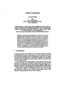
Fig. 3. A flow from s to t. For convenience, the arc (t, s) is omitted. All arcs have a minimum capacity of 0 and a maximum capacity of 1, excepted the outgoing arcs from s where the capacities are given in parenthesis. For instance, the arc (s, D) has a minimum capacity equals to 1 and a maximum equals to 2.

♢ Flow Computation Consider, for instance, that all the lower bounds are equal to zero and suppose that you want to increase the flow value for an arc (i, j). In this case, the flow of zero on all arcs, called the zero flow, is a feasible flow. Let P be a path from j to i different from [j, i], and val = min({uij } ∪ {upq s.t. (p, q) ∈ P }). Then we can define the function f on the arcs of G such that fpq = val if P contains (p, q) or (p, q) = (i, j) and fpq = 0 otherwise. This function is a flow in G. (The conservation law is obviously satisfied because (i, j) and P form a cycle.) We

peter paul mary t

john bob mike julia Orientation :

M (1,2) D (1,2) N (1,1)

s

B (0,2) O (0,2) bold edge thin edge

Fig. 4. The residual graph for the flow given in Figure 3.For convenience, the arc (t, s) and (s, t) are omitted. All arcs have a minimum capacity of 0 and a maximum capacity of 1.

have fij > 0, hence it is easy to improve the flow of an arc when all the lower bounds are zero and when we start from the zero flow. It is, indeed, sufficient to find a path satisfying the capacity constraint. The main idea of the basic algorithms of flow theory, is to proceed by successive modifications of flows, that are computed in a graph in which all the lower bounds are zero and the current flow is the zero flow. This particular graph can be obtained from any flow and is called the residual graph: Definition 2 The residual graph for a given flow f , denoted by R(f ), is the digraph with the same node set as in G. The arc set of R(f ) is defined as follows: ∀(i, j) ∈ U (G): • fij < uij ⇔ (i, j) ∈ U (R(f )) and upper bound capacity rij = uij − fij . • fij > lij ⇔ (j, i) ∈ U (R(f )) and upper bound capacity rji = fij − lij . All the lower bound capacities are equal to 0.

Figure 3 and Figure 4 are examples of flow and residual graph of the example given in Figure 2. Instead of working with the original graph G, we can work with the residual graph R(f o ) for some f o . From f ′ a flow in R(f o ), we can obtain f another flow o ′ ′ in G defined by: ∀(i, j) ∈ U (G) : fij = fij + fij − fji . And from a path in R(f o ) ′ o we can define a flow f in R(f ) and so a flow in G: Definition 3 We will say that f is obtained from f o by sending k units of flow along a path P from j to i if: o • P is a path in R(f ) − {(j, i)} • k ≤ min({rij } ∪ {ruv s.t.(u, v) ∈ P }) o ′ • f corresponds in R(f ) to the flow f defined by: ′ • f pq = k for each arc (p, q) ∈ P ∪ {(i, j)}

′ fpq = 0 for all other arcs. If k is not mentioned it will be assumed that k = min({rij }∪{ruv s.t.(u, v) ∈ P }) •

In the previous definition the path must be different from [j, i], otherwise f ′ will be the zero flow. The following proposition shows that the existence of a path in the residual graph is a necessary and sufficient condition: Theorem 1 Let f o be any feasible flow in G, and (i, j) be an arc of G. o • There is a feasible flow f in G with fij > f ij if and only if there exists a o path from j to i in R(f ) − {(j, i)}. o • There is a feasible flow f in G with fij < f ij if and only if there exists a o path from i to j in R(f ) − {(i, j)}. proof: see [79] p112. ⊙

♢ Maximum flow algorithm Theorem 1 gives a way to construct a maximum flow in an arc (i, j) by iterative improvement, due to Ford and Fulkerson: Begin with any feasible flow f 0 and look for a path from j to i in R(f 0 )−{(j, i)}. If there is none, f 0 is maximum. If, on the other hand, we find such a path P , then define f 1 obtained from f 0 by sending flow along P . Now look for a path from j to i in R(f 1 ) − {(j, i)} and repeat this process. When there is no such path for f k , then f k is a maximum flow. A path can be found in O(m), thus we have2 : Property 3 A maximum flow of value v in an arc (i, j) can be found from a feasible flow in O(mv). ♢ Feasible flow algorithm For establishing a feasible flow, several methods exist. For instance, it is possible to transform this problem into one in which all the lower bounds capacities are equal to zero and searching for a particular maximum flow value for one arc. (See [2] p 169.) However, there is a simple method which repeatedly searchs for maximum flows in some arcs: Start with the zero flow f o . This flow satisfies the upper bounds. Set f = f o , and apply the following process while the flow is not feasible: 1) pick an arc (i, j) such that fij violates the lower bound capacity in G (i.e. fij < lij ). 2) Find P a path from j to i in R(f ) − {(j, i)}. 3) Obtain f ′ from f by sending flow along P ; set f = f ′ and goto 1) If, at some point, there is no path for the current flow, then a feasible flow does not exist. Otherwise, the obtained flow is feasible. 2

This complexity comes from the integer capacities. In this case, the flow is augmented by at least one for each iteration.

Property 4 Let kij be the infeasibility number w.r.t. the zero flow of each arc (i, ∑j) in G. We can find a feasible flow in G or prove there is none in O(m (i,j)∈U (G) kij ). ♢ Flow properties The most interesting property for us is a Corollary of Theorem 1. Corollary 2 Let f o be any feasible flow in G, and (i, j) be an arc of G. The flow value fij is constant for any feasible flow f if and only if: o • there is no path from j to i in R(f ) − {(j, i)}; and o • there is no path from i to j in R(f ) − {(i, j)}. We will also consider a specific case which is useful for our purpose: Corollary 3 Let f o be any feasible flow in G, and (i, j) be an arc of G with o = 0. The flow value fij is equal to 0 for any feasible flow f if and only if i fij and j belong to two different strongly connected component of R(f o ) The search for strongly connected components can be done in O(m + n + d) [143]. The advantage of this proposition is that all the arcs (i, j) with a constant 0 flow value can be identified by only one identification of the strongly connected components in R(f o ). This corollary is used in the following way: suppose that i represents a variable and j a value of i. Now, if the constraint is equivalent to the search of a feasible flow in a graph which contain an arc from i to j iff j belongs to the domain of i then if the corollary gives us a necessary and sufficient condition to determine if (i, j) is consistent with the constraint. This is exactly the reasoning used for the global cardinality constraint as we will see later in this chapter. Alldiff and Permutation Constraints (alldiff,permutation) The alldiff constraint constrains the values taken by a set of variables to be pairwise different. The permutation constraint is an alldiff constraint in which |D(X(C))| = |X(C)|. Definition 4 An alldiff constraint is a constraint C defined by alldiff(X) = {τ s.t. τ is a tuple on X(C) and ∀ai ∈ D(X(C)) : #(ai , τ ) ≤ 1} This constraint is used in a lot of real world problems like rostering or resource allocation. It is quite useful to express that two things cannot be at the same place at the same moment. A filtering algorithm establishing arc consistency for the alldiff is given in ∑ [107]. Its complexity is in O(m) with m = x∈X |D(x)|, after the computation √ of the consistency of the constraint which requires O( nm). When the domain of

the variables are intervals, [90] proposed a filtering algorithm establishing bound consistency with a complexity which is asymptotically the same as for sorting the internal endpoints. If the interval endpoints are from an integer range of size O(nk ) for some constant k the algorithm runs in linear time. Therefore, Melhorn’s algorithm is linear for a permutation constraint. Lopes et al. [85] have designed an original and simple algorithm having the same complexity. A comparison between several algorithms is available in [141]. On the other hand, [81] has proposed an algorithm which considers that the domains are intervals, but which can create “holes” in the domain, that is the resulting domain will be union of intervals. His filtering algorithm is in O(n2 d). In the original paper, Régin’s filtering algorithm is based on matching theory, but we can also use the flow theory in order to obtain almost the same algorithm. We will not describe this algorithm here, because we prefer to detail a more general constraint : the global cardinality constraint. From this constraint we can immediately obtain a filtering algorithm for the alldiff constraint. Global Cardinality Constraint (gcc) A global cardinality constraint (gcc) constrains the number of times every value can be taken by a set of variables. This is certainly one of the most useful constraints in practice. Note that the alldiff constraint corresponds to a gcc in which every value can be taken at most once. Definition 5 A global cardinality constraint is a constraint C in which each value ai ∈ D(X(C)) is associated with two positive integers li and ui with li ≤ ui defined by gcc(X, l, u) = { τ s.t. τ is a tuple on X(C) and ∀ai ∈ D(X(C)) : li ≤ #(ai , τ ) ≤ ui } This constraint is present in almost all rostering or car-sequencing problems. A filtering algorithm establishing arc consistency for this constraint has been proposed by Régin [109]. The consistency of the constraint can be checked in O(nm) and the arc consistency can be computed in O(m) providing that a maximum flow has been defined. Two other algorithms establishing bound consistency for this constraint have been developed by Quimper et al. [102] and Katriel et al. [71]. The first one is original whereas the second is an adaptation of Régin’s algorithm [109]. We propose to describe Régin’s algorithm here. This algorithm is mainly based on the following observation: a gcc C is consistent iff there is a flow in an directed graph N (C) called the value network of C [109]: Definition 6 Given C = gcc(X, l, u) a gcc; the value network of C is the directed graph N (C) with lower bound capacity and upper bound capacity on each arc. N (C) is obtained from the value graph GV (C), by:

• orienting each edge of GV (C) from values to variables. For such an arc (u, v): luv = 0 and uuv = 1. • adding a node s and an arc from s to each value. For such an arc (s, ai ): lsai = li , usai = ui . • adding a node t and an arc from each variable to t. For such an arc (x, t): lxt = 1, uxt = 1. • adding an arc (t, s) with lts = uts = |X(C)|.

Figure 3 and Figure 4 are examples of flow and residual graph of the example of the gcc given in Figure 2. Proposition 2 Let C be a gcc and N (C) be the value network of C; the following two properties are equivalent: • C is consistent; • there is a feasible flow in N (C). sketch of proof: We can easily check that each tuple of T (C) corresponds to a flow in N (C) and conversely. ⊙

From Corollary 3 we immediately have: Proposition 3 Let C be a consistent gcc and f be a feasible flow in N (C). A value a of a variable x is not consistent with C if and only if fax = 0 and a and x do not belong to the same strongly connected component in R(f ). For our problem, a feasible flow can be computed in O(nm) therefore we have the same complexity for the check of the constraint consistency. Moreover flow algorithms are incremental. The search for strongly connected components can be done in O(m + n + d) [143], thus a good complexity for computing arc consistency for a gcc is obtained. Corollary 4 Let C be a consistent gcc and f be a feasible flow in N (C). Arc consistency for C can be established in O(m + n + d). Here is a recapitulation of the complexities: Consistency Arc consistency From scratch O(n m) O(m + n + d) After k modifications O(k m) O(m + n + d)

Cardinality Matrix Constraint (card-matrix) This constraint has been proposed by Régin and Gomes [120]. Cardinality matrix problems are the underlying structure of several real world problems such as rostering, sports scheduling , and timetabling. These are hard

computational problems given their inherent combinatorial structure. The cardinality matrix constraint takes advantage of the intrinsic structure of the cardinality matrix problems. It uses a global cardinality constraint per row and per column and one cardinality (0,1)-matrix constraint per symbol. This latter constraint corresponds to solving a special case of a network flow problem, the transportation problem, which effectively captures the interactions between rows, columns, and symbols of cardinality matrix problems. In order to show the advantage of this constraint, consider a restricted form of the cardinality matrix problems: the alldiff matrix problem[59]. In this case, each value has to be assigned at most once in each row and each column. The alldiff matrix characterizes the structure of several real world problems, such as design of scientific experiments or fiber optics routing. Consider the following example: a 6x6 matrix has to be filled with numbers ranging from 1 to 6 (this is a latin square problem). A classical model in CP consists of defining one variable per cell, each variable can take a value from 1 to 6, and one alldiff constraint per row and one alldiff constraint per column. Now, consider the following situation: 1 2 3 4 • • • •

2 1 4 5 • • • •

In this case, the alldiff constraints are only able to deduce that: • only the values 5 and 6 can be assigned to the cells (5, 3) and (6, 3) • only the values 3 and 6 can be assigned to the cells (5, 4) and (6, 4). However, with a careful study we can see that the value 6 will be assigned either to (5, 3) and (6, 4) or to (5, 4) and (6, 3) this means that the other columns of rows 5 and 6 cannot take these values and therefore we can remove the value 6 from the domains of the corresponding variables (the ones with a • in the figure). The cardinality (0,1)-matrix, automatically performs these inferences. Definition 7 A cardinality matrix constraint is a constraint C defined on a Matrix M = x[i, j] of variable s taking their values in a set V , and on two sets of cardinality variables rowCard[i, j] and colCard[i, j] and card-Matrix(M, V, rowCard, colCard) = { τ s.t. τ is a tuple on X(C) and ∀ak ∈ V, ∀i ∈ Row(M ) : #(ak , vars(i, ∗, M )) = rowCard[i, k] and ∀ak ∈ V, ∀j ∈ Col(M ) : #(ak , vars(i, ∗, M )) = colCard[j, k]} If the matrix is form only by (0,1)-variable then we say that we have a (0,1)matrix. Régin and Gomes proposed an AC filtering algorithm for matrix variables of the card-(0,1)-Matrix constraint by a similar method to the one used for

gccs[120]. A similar constraint, althrough expressed in a quite different way, with the same kind of algorithm to establish arc consistency, is given in [74]. Experimental results have shown that the card-matrix constraint outperforms standard constraint based formulations of cardinality matrix problems. Global Cardinality Constraint with Costs (cost-gcc) A global cardinality constraint with costs (cost-gcc) is the conjunction of a gcc constraint and a sum constraint: Definition 8 A cost function on a variable set X is a function which associates with each value (x, a), x ∈ X and a ∈ D(x) an integer denoted by cost(x, a). Definition 9 A global cardinality constraint with costs is a constraint C associated with cost a cost function on X(C), an integer H and in which each value ai ∈ D(X(C)) is associated with two positive integers li and ui ; and defined by cost-gcc(X, l, u, cost, H) = { τ s.t. τ is a tuple on X(C) and ∀ai ∈ D(X(C)) : li ≤ #(ai , τ ) ≤ ui |X(C)| and Σi=1 cost(var(C, i), τ [i]) ≤ H } This constraint is used to model some preferences between assignments in resource allocation problems. Note that there is no assumption made on the sign of costs. The integration of costs within a constraint is quite important, especially to solve optimization problems, because it improves back-propagation, which is due to the modification of the objective variable. In other words, the domain of the variables can be reduced when the objective variable is modified. [38] have used an alldiff constraint with costs, but only the consistency of the constraint has been checked, and no specific filtering has been used. The first proposed filtering algorithm comes from [49] and [50], and is based on reduced cost. A filtering algorithm establishing arc consistency has been proposed by Régin [111, 113]. The consistency of this constraint can be checked by searching for a minimum cost flow and arc consistency can be established in O(|∆|S(m, n + d, γ)) where |∆| is the number of values that are taken by a variable in a tuple, and where S(m, n + d, γ)) is the complexity of the search for shortest paths from a node to every node in a graph with m arcs and n nodes with a maximal cost γ. 3.3

Balancing Constraints

Pesant and Régin introduced the notion of balancing constraints [96]. Many combinatorial problems require of their solutions that they achieve a certain balance of given features. Balance is often important in assignment problems or in problems with an assignment component. We give a few examples. In

assembly line balancing the workload of the line operators must be balanced. In rostering we may talk of fairness instead of balance, because of the human factor. Here we want a fair distribution of weekends off or of night shifts among workers, for example. In vehicle routing one dimension of the problem is to partition the customers into the different routes - balancing the number of customers served on each route, the quantity of goods delivered, or the time required to complete the route may be of interest. We could describe the balance in the following way: • the average value should be close to a given target, corresponding to the ideal value; • there should be no outliers, as they would correspond to an unbalanced situation; • values should be grouped around the average value. Pesant and Régin claimed that statistics provide appropriate mathematical concepts to express this and they proposed the first constraints based on statistic: the spread constraint and bound consistency filtering algorithms associated with it. Roughly, the spread constraint is defined on a set of numerical variables and combines the mean of these variables with the standard deviation. Schaus et al. noticed that this idea can be generalized to the concept of Lp norm [129, 128, 130]. Definition 10 Let X = {x1 , x2 , ..., xn } be a set of n variables, µ be ∑ a variable, n L be a cost variable and the Lp (X, µ)-norm defined as Lp (X, µ) = [ i=1 |xi − 1 µ|p )] p . The balance constraint is the constraint C defined on X, {µ} and L, and ∑ associated with a value of p such that C holds if and only if Lp (X, µ) = L n and i=1 xi = nµ where the different norm are: • L0 = |{x ∈ X s.t. x ̸= µ is the number of values different from the mean ∑ • L1 = ∑x∈X |x − µ| 2is the sum of deviations from the mean • L2 = x∈X (x − µ) is the sum of square deviations from the mean • L∞ = maxx∈X |x − µ| is the maximum deviation from the mean it is denoted by balance(X, µ, L, p) Note that the balancing constraint considers the two sums simultaneously. None of these balance criteria subsumes the others. For instance, the minimization of L1 does not imply in general a minimization of criterion L2 . This is illustrated on the following example. Assume a constraint problem with four solutions given in Figure 5. The most balanced solution depends on the chosen norm. Each solution exhibits a mean of 100 but each one optimizes a different norm. Choosing the "best" criteria is an old question which has no definitive answer. Pesant and Régin considered the case where p = 2 and named the constraint spread. They gave a bound consistency filtering algorithm for the X variables in O(n2 ). Note that the spread constraint in its general form considers µ and L (i.e. σ) as variables and not constant. Then, Schaus et al. proposed to simplify the algorithm when µ is a given constant [129]. They also derived some other

sol. num. 1 2 3 4

solution 100 100 100 100 30 170 60 80 100 100 120 140 70 70 90 110 130 130 71 71 71 129 129 129

L0 2 4 6 6

L1 140 120 140 174

L2 9800 4000 3800 5046

L∞ 70 40 30 29

Fig. 5. Illustration showing that no balance criterion defined by the norm L0 , L1 , L2 or L∞ subsumes the others. The smallest norm is indicated in bold character. For example, solution 2 is the most balanced according to L1 .

filtering algorithms for L, X and µ. Having µ as a constant is quite frequent in practice. However, this is not always the case, for instance when X variables measures a slack or an overflow, the ideal should be to have no overflow, so 0 for the mean, but we do not have negative x, because it has no practical meaning (an underflow does not compensate an overflow). Next, Schaus et al. studied the deviation constraint, that is the balance constraint with p = 1 [128]. They proposed efficient bound consistency filtering algorithms (in O(n)) when considering the mean as a constant value. Further investigations and recent developments can be found in Schaus’s PhD thesis [127]. 3.4

Constraint Combination based Constraints

Max-SAT constraint (max-sat) A lot of work have been carried out in order to improve the computation of minimization of the number of violated constraints in an over-constrained problem (Max-CSP). Several algorithms have been designed. First, Partial Forward Checking [51], which has been improved by PFC-DAC [155, 78], then by PFC-MRDAC [77]3 . The major drawback of these algorithms is that there are ad-hoc algorithms based on a branch-and-bound procedure and they mainly consider only binary constraints. Therefore, their integration into a CP Solver is not easy. Thus, Régin et al. have proposed to define a constraint corresponding to this specific problem like any other global constraint [121]. Definition 11 Let C = {Ci , i ∈ {1, . . . , m}} be a set of constraints, cost(C) be a set of cost variables associated with the constraints of C and unsat a variable. A Max-SAT constraint is a constraint ssc(C, cost(C), unsat) defined by the conjunction of the constraint ∑ unsat = cost(C) C∈C 3

This algorithm can be viewed as a generalization of the constructive disjunction in the case where several constraints must be satisfied and not only one.

and the set of disjunctive constraints {[(C ∧ (cost(C) = 0)) ∨ (C ∧ (cost(C) = 1))], C ∈ C} It is denoted by max-sat(C) Then Régin et al. integrated some classical algorithms defined for solving over-constrained problem as filtering algorithm of this global constraint. Let P = (X, D, C) be a constraint network. Notation 1 ∗ • v (P ) is the number of violated constraint of P ∗ • v(P ) is any lower bound of v (P ) ∗ • v ((x, a), P ) is the number of violated constraints of P when x = a ∗ • v((x, a), P ) is any lower bound of v ((x, a), P ) Definition 12 Two sub-problems Q1 = (X, D, K) and Q2 = (X, D, L) of P are constraint disjoint iff K ∩ L = ∅ Theorem 2 (Régin et al.) Given P = (X, D, C) a constraint network and Q et set of sub-problems of P that are pairwise constraint disjoint then : ∑ ∑ v ∗ (P ) ≥ v ∗ (Q) ≥ v(Q) Q∈Q

Q∈Q

Then we have two corollaries: Corollary 5 Let obj be a value. If of P with v ∗ (P ) ≤ obj

∑ Q∈Q

v(Q) > obj then there is no solution

Corollary 6 Let obj be ∑ a value and a be a value of a variable x involved in a sub-problem Q of Q. If R∈(Q−Q) v(R) + v((x, a), Q) > obj then there is no solution of P with v ∗ ((x, a), P ) ≤ obj This corollary will permit to remove some inconsistent values. The main issue is the computation of a set Q and the choice of v(Q) for a given problem Q. Régin et al. noted that PFC-MRDAC algorithm proposes, in fact, to build the set Q in the following way: we begin with the set of constraints K = C and we order the variables (with any order). Then, we select the variable in that order. When a variable x is selected we take all the constraints of K involving x in order to create a sub-problem denoted by Q(x) and we remove from K these constraints before considering the next variable. From the specific construction of Q we obtain a value of v(Q) which is easy to compute: since each sub-problem is defined from a variable x which is involved in all the constraints of the sub-problem, we can compute for each value a of x the number of constraints violated if x = a, and we define v(Q) as the value

having the smallest number of violations. This information can be maintained efficiently. Then several improvements of this integration , and so also of PFC-MRDAC algorithm, have been proposed notably to deal efficiently with interval variables [122, 98]. At last, a new algorithm based on conflict set has been proposed [122]. A conflict set is a set of constraints which is inconsistent. Some information about this constraint can also be found in Régin’s HDR thesis [117]. Or and And constraints (and,or) Lhomme [83] studied the logical combination of constraints, sometimes called meta-constraints because it noticed that although these constraints are extremely useful for modelling problems, they have either poor filtering algorithms or are not very efficient. First, Lhomme considered the constraint or(C1 , C2 ) which is satisfied if C1 is satisfied or if C2 is satisfied. He showed that the constructive disjunction (See [149] for more information) establishes arc consistency for this constraint but constructive disjunction is complex to implement and not very efficient. Hence he proposed another algorithm much more efficient. It is based on the following remarks: • Let x be a variable involved in C1 and in C2 . If we find a support for (x, a) on C1 then it is useless to search for a support for (x, a) on C2 because (x, a) satisfies the disjunction (i.e. has a support on at least one constraint) • It is useless to search for supports for variables of X(C2 ) that are not in X(C1 ), because C1 can be true and in this case all the values of these variables are consistent with the or constraint. The same reasoning applied for variables of X(C1 ) that are not in X(C2 ). Therefore, Lhomme established the following Proposition: Proposition 4 Let C =or(C1 , C2 ) be the constraint equals to the disjunction between the constraint C1 and the constraint C2. Then, C is arc consistent if and only if the values of the variables of (X(C1 ) ∩ X(C2 )) are consistent either with C1 or with C2 . Lhomme also addressed the constraint equivalent to the conjunctions of two constraints C1 and C2 . We have already mentioned the difference between establishing arc consistency for the constraints taken separately and for the constraint C =and(C1 , C2 ). Lhomme proposed an algorithm based on the simultaneous search for support for the variables involved in both constraints. Unfortunately such a search imposes the availability of some functions for each constraints which is rarely the case. However, this is the case for table constraints given in extension and Lhomme gave an algorithm for them. The principles given in this section can be easily generalized to combinations of several constraints and not only two.

3.5

Sequencing Constraints

Sequencing constraints are useful in rostering or car sequencing problems to constrains the number of time some values are taken by any group of k consecutive variables. For instance, they are used to model that on an assembly line, at most one car over three consecutive cars can have a sun roof. They are based on a conjunction of among constraints, which are defined as follows Among Constraint (among) Definition 13 Given X a set of variables, l and u two integers with l ≤ u and V a set of values. The among constraint ensures that at least l variables of X and at most u will take a value in V , that is ∑ among(X, V, l, u) = {t | t is a tuple of X and l ≤ a∈V #(a, τ ) ≤ u} This constraint has been introduced in CHIP [17]. It is straightforward to design a filtering algorithm establishing arc consistency for this constraint. For instance, we can associate with each variable xi of X a (0, 1) variable yi defined as follows: yi ∑ = 1 if and only if xi = a with a ∈ V . Then the constraint can be rewritten l ≤ yi ≤ u. Note that the among constraint is sometimes directly defined in that way, that is by involving only this set Y of (0, 1) variables. The sequence constraint is a conjunction of gliding among constraints. Sequence Constraint (sequence) Definition 14 Given X a set of variables, q, l and u three integers with l ≤ u and V a set of values. The sequence constraint holds if and only if for 1 ≤ i ≤ nq + 1 among({xi , ..., xi+q−1 }, V, l, u) holds. More precisely Sequence(X, V, q, l, u) = { t | t is a tuple of X and for each ∑ sequence S of q consecutive variables: l ≤ v∈V #(v, t, S) ≤ u} This constraint has been introduced in CHIP [17]. Several filtering algorithms have been proposed for this constraint. First, it is possible to use only the set of overlapping among constraints, but this does not lead to efficient domain reductions. The card-path constraint of Beldiceanu and Carlsson can also be used [10]. However, the filtering algorithm does not establish arc consistency. Some pseudo polynomial algorithms for establishing have been designed. Bessiere et al. [27] gave a domain consistency propagator that runs in O(nqdq ) time. van Hoeve et al. [152] proposed an encoding into a regular constraint which runs in O(n2q ) time. The first strongly polynomial algorithm (in O(n3 )) establishing arc consistency has been proposed by van Hoeve et al. [152, 153]. Then, several polynomial algorithms with different complexities have been introduced by Brand et al. [33] and, at last, a very nice model leading to the best filtering algorithm is described in [87]. We propose to describe quickly some of these algorithms because it is rare to obtain several algorithms while using different approaches, and this could be useful for some other constraints.

For the sake of clarity, we will use the two equivalent representations of the among constraint. The one using the X variable set and the other using the Y variable set. First, van Hoeve et al. [152] remarked that when l is equal to u then arc consistency can be established in linear time. In this case, in any solution xi will be equal to xi+q because two [?] constraints ensure that yi + ...yi+q−1 = l and yi+1 + ...yi+q = l. So, by adding these new equality constraints and by using the filtering algorithm associated with each among constraint, arc consistency will be established by the propagation mechanism. Then, three strongly polynomial filtering algorithms establishing arc consistency have been proposed. There are based on different concepts: cumulative sum, difference constraint and flow. FA based on cumulative sum A set of n + 1 new variables si are introduced. A variable si correspond to the sum of the yj variables for j = 1 to i. The S variables are encoded as follows: s0 = 0 and si = yi + si−1 . Then, the constraints sj ≤ sj+q − l and sj+q ≤ sj + u for 1 ≤ j ≤ n − q + 1 are added to the model. Brand et al. [33] have proposed this model and shown that enforcing singleton bound consistency on these variables establishes arc consistency for the sequence constraint. In addition, they proved that the complexity of maintaining arc consistency on a branch of the tree search is in O(n3 ). This model is also a reformulation (and an improvement) of the first filtering algorithm establishing arc consistency in polynomial time of van Hoeve et al. [152, 153]. FA based on difference constraint This approach uses difference constraints, that is constraints of the form S ≤ S ′ + d, for encoding the sequence constraint. It has been proposed by Brand et al. [33] and it uses the S variables like in the previous approach, but the constraint si = yi + si−1 is replaced by the two equivalent constraints si−1 ≤ si ≤ si−1 + 1 and yi ⇔ si−1 ≤ si − 1. The consistency of a set of distance constraints can be checked by searching for the presence of negative cycle in a graph (see [42] or [39] section 24.4). Thus, an AC filtering algorithm can be simply derived by using the current assignment of the Y variables in order to define the set DC of distance constraints. After checking the consistency of DC, the boundaries of the Y variables are explicitly tested. That is, if DC implies that si−1 ≤ si − 1 then yi = 1 and if DC implies that si ≤ si−1 then yi = 0. The authors show that this FA can be maintained during the search with a complexity on a branch of the tree search in O(n2 log(n)).

FA based on flow This clever approach has been proposed in [87]. The idea is to represent a sequence constraint by an integer linear program formed by the among constraints it contains. Then, the specific structure of the obtained matrix (it has the consecutive ones property for the column) is exploited and the model is transformed into a network flow problem. Thus, the computation of some properties of the flow problem, like the constant arc for all feasible flow, leads to an AC filtering algorithm. This approach has two main advantages: the problem is just transformed into a flow problem and so there is no need to write any specific algorithms; and the complexity is reduced. This FA, indeed, can be maintained during the search with a complexity on a branch of the tree search in O(n2 ). Maher et al. use an existing transformation from matrix having the consecutive ones property to a network flow problem. This transformation is explained in [2] and leads to a flow which is not really easy to understand. We propose here to try to directly explain the obtained flow.

t

TB

T12

W1

T23

W2

T34

W3

T45

W4

T56

W5

TE

W6

s

Fig. 6. The graph associated with a sequence problem.

Consider the following problem: 9 variables from x1 to x9 , a sequence of width 4, l = 1, and u = 3, meaning that at least one variable and at most 3 variables of each sequence of 4 consecutive variables must be set to 1. Figure 6. The graph on which the flow is defined is built as follows: First we define the nodes: • we create a source s and a sink t. • we create as many W-nodes as there are complete sequences. For the example, we have 6 complete sequences, so we create 6 W-nodes: w1 , ..., w6 . A W-node is a windows node and corresponds to a sequence. Node W 1 represents the sequence x1 , x2 , x3 , x4 , node W 2 the sequence W 2, W 3, W 4, W 5 etc... • we create as many T-node as there are non empty intersection between consecutive W-nodes and we add 2 special T-node: TB and TE. A T-node is a transition node and represents what two W-nodes have in common. Node T 12 corresponds to the W-nodes W 1 and W 2, node T 23 corresponds to the W-nodes W 2 and W 3 etc... Node TB corresponds to the beginning of the sequence and node TE to the end of the sequence Then, we define the arcs: • there is an arc from t to s. • there is an arc between s and each W-node. The required quantity of flow (i.e. the flow must be equal to this value) in each arc is [u − l] corresponding to the slack we have for sequence from the minimum (i.e. l). • there is an arc between from each T-node but TB to t. The required quantity of flow in each arc is [u − l] corresponding to the slack we have a sequence from the minimum (i.e. l), excepted for TE for which the required quantity of flow is u. • there is an arc between s and TB. The required quantity of flow in this arc is l. The idea is that each sequence must have at least l units of flow. TB is used to receive this quantity and then to transmit it to the other T-nodes. • there is an arc between any W-node and the two T-nodes associated with it. Node W i is linked to T-node T (i − 1)i and node T i(i + 1). W 1 is linked to TB and T 12 and W 6 is linked to T 5 and T E. All these arcs have are (0,u-l) arcs (the flow traversing them has a value in [0, u − l]). • there are arcs between T-nodes. Each T-node T i(i + 1), excepted TB and TE, has one entering arc and one leaving arc. The entering arc represent the variable which is in W i but not in W (i + 1) and the leaving arc represents the variable which is in W (i + 1) and not in W i. For instance, the arc from T 12 to T 56 represents variable x5 . TB has 4 (the width) leaving arcs corresponding to the 4 first variables x1 , x2 , x3 , x4 and TD has 4 entering arcs corresponding to the 4 last variables x6 , x7 , x8 , x9 . All these arc are (0,1) arcs and their flow value corresponds to the value of the variable in any solution. Now, a feasible flow in this graph corresponds to a solution of the problem. The intuitive idea is that we send the minimum unit of flow TB and this quantity of flow will be propagated to the sequences thanks to arcs defined by x variables. The arcs leaving s and entering t are then to ensures the flow conservation and

to express the fact that some sequences have more 1 than others. Then arc consistency of the variables x is computed by searching for constant values for the arcs corresponding to these variables, which can be done thanks to Corollary 2 (See Flow Properties). Figure 7 shows an example of feasible flow for some values of x variables. The arc having a constant flow value equal to 0 have been removed.

t

TB

T12 2

W1

T23 1

W2

T34

1

2

T45 1

W3

W4

1

T56 2

W5

1,2

TE 0,1

0,1

W6

s

Fig. 7. A feasible flow when x1 = 0,x2 = {0, 1},x3 = 0,x4 = 0,x5 = 1,x6 = {0, 1},x7 = 1,x8 = 1,x9 = {0, 1}. The arcs that cannot carry any unit of flow in any feasible flow have been removed. Number indicates the flow value. There are separated by comma when there are several possible flow values for other solutions

Some experiments given in [33, 87] show that the algorithms based on cumulative sums and the flows are the best in practice. The latter one seems to be more robust. Some generalizations or variations of the sequence constraint have also been studied.

Generalized Sequence Constraint (gen-sequence) This constraint generalizes the sequence constraint by adding some other among constraints. These among constraints must be defined using the same set of value V than the sequence. Definition 15 Given X an ordered set of variables, Q a set of ordered subset of X (i.e subset of consecutive variables of X) where each subset Qi is associated with two numbers li and ui and V a set of values. The generalized sequence constraint constraint holds if and only if for each Qi ∈ Q among(Qi , V, li , ui ) holds. More precisely gen-sequence(X, V, Q, {li }, {ui }) = { t | t ∑ is a tuple of X and ∀Qi ∈ Q li ≤ v∈V #(v, t, Qi ) ≤ ui } This constraint has been proposed by van Hoeve et al. [152]. The authors gave a FA establishing arc consistency for it, whose complexity is in O(n4 ). This algorithm is based on the same idea as the cumulative sum for the sequence constraint. However, Maher et al. [87] also considered this constraint in order to try to apply the modeling idea of representing the constraint by a flow. Sometimes, the obtained matrix satisfies the consecutive one property and the method can be applied and so a quadratic AC filtering algorithm exists. It is also possible that the matrix will satisfy the consecutive one property if the subset of X are reordered. Such a result can be obtained in polynomial time (see [87]). However, for some matrices it will not be possible to obtained the desired property. In this case, an encoding based on difference can be used leading to an AC Filtering algorithm whose complexity is in O(nm + n2 log(n)) for any branch of the tree search, where m is the number of element of Q.

Global Sequencing Constraint (gsc) The global sequencing constraint (gsc) has been designed mainly to try to solve some car sequencing instances. It combines a sequence constraint and global cardinality constraints. A global sequencing constraint C is specified in terms of a ordered set of variables X which take their values in D, some integers q, min and max and a given subset V of D. On one hand, a gsc constrains the number of variables in X instantiated to a value vi ∈ D to be in an interval [li , ui ]. On the other hand, a gsc constrains for each sequence Sj of q consecutive variables of X(C), that at least min and at most max variables of Sj are instantiated to a value of V . Definition 16 Given X an ordered set of variables, m, M, q three positive integers, a set of values D in which each value ai ∈ D is associated with two positive integers li and ui , and a set of values V . The global sequencing constraint

is defined by gsc(X, D, {li }, {ui }, V, m, M, q) = { t | t is a tuple of X and ∀ai ∈ D : li ≤ #(ai , t) ≤ ui and for each sequence S of q consecutive ∑ variables: m ≤ vi ∈V #(vi , t, S) ≤ M } This constraint has been proposed by Régin [123]. It arises in car sequencing or in rostering problems. A filtering algorithm is described in [123]. It is based on the reformulation of the problem mainly using flows and it has been implemented in ILOG Solver. Thanks to it, some problems of the CSP-Lib have been closed and a recent and nice experimental study of [153] shows that this constraint leads to good results for solving some car sequencing instances of the CSP-Lib. In fact 12 problems are solved by a CP model only if it uses this constraint. About sequencing constraints, some other combinations of among constraints with or without cardinality constraints have been considered. For instance, Régin [118] studied several combinations of among constraints. He mainly showed that in general a combination of among constraints is an NP-Complete problem. Nevertheless, if the among constraints are pairwise value disjoint (i.e. the set of values associated with each among constraint are disjoint), then it is possible to represent the set of among constraints by a unique gcc and so to obtain a polynomial AC filtering algorithm. In addition, Régin proposed some kind of shaving or singleton arc consistency to improve the combination of among and cardinality constraints. He applied his result to the inter-distance constraint. At last, we need to mention two other variations of the sequencing constraints have been recently considered: the multiple sequence and the sliding-sum. The multiple sequence has been introduced in [33] and combines several sequence constraints provided that the values counted by each sequence are pairwise disjoint. Then, an AC filtering algorithm based on the regular constraint has been proposed. The sliding-sum has been introduced by Beldiceanu [9] and is a generalization of the sequence constraint to non (0,1) variables, that is the sum of variable is directly considered. An efficient bound consistency filtering algorithm has been proposed for this constraint in [87].

3.6

Distance Constraints

Inter-distance Constraint (inter-distance) Régin [110] introduced, under the name "Global Minimum Constraint", a constraint defined on X a set of variables stating that for any pair of variable x and y of X the constraint |x − y| ≥ k is satisfied. This constraint is mentioned in [63].

Definition 17 An inter-distance constraint is a constraint C associated with an integer k and defined by inter-distance(k) = { τ s.t. τ is a tuple of X(C) and ∀ai , aj ∈ τ : |ai − aj | ≥ k} This constraint is present in frequency allocation problems or in scheduling problems in which tasks require p contiguous units of resource to be completed. A filtering algorithm has been proposed for this constraint [110]. Note that there is a strong relation between this constraint and the sequence constraint. An 1/q sequence constraint constrains two variables assigned to the same value to be separated by at least q − 1 variables, in regard to the variable ordering. Here, we want to select the values taken by a set of variables such that are all pairs of values are at least k units apart. Then, a bound consistency algorithm has been proposed by Artiouchine and Baptiste [5, 6]. This algorithm runs in O(n3 ). It has been improved later by Quimper et al. [101] for running in O(n2 ). Sum and Binary Inequalities Constraint (sum-ineq) This constraint is the conjunction of a sum constraint and a set of distance constraints, that is constraints of the form xj − xi ≤ c. Definition 18 Let SU M (X, y) be a sum constraint, and Ineq be a set of binary inequalities defined on X. The sum and binary inequalities constraint is a constraint C associated with SU M (X, y) and Ineq defined by: sum-ineq(X, y, Ineq ) = { τ s.t. τ is a tuple of X ∪ y ∑|X| and ( i=1 τ [i]) = τ [y] and the values of τ satisfy Ineq } This constraint has been proposed by Régin and Rueher [124]. It is used to minimize the delays in scheduling applications. Bound consistency can be computed in O(n(m+n log n)), where m is the number of inequalities and n the number of variables. It is also instructive to remark that i=n the bound consistency filtering algorithm still works when y = Σi=1 αi xi where αi are non-negative real numbers. 3.7

Geometric Constraints

the most famous geometric constraint is the diff-n constraint. We quote [17]: “The diff-n constraint was introduced in CHIP in order to handle multi-dimensional placement problems that occur in scheduling, cutting or geometrical placement problems. The intuitive idea is to extend the alldiff constraint which works on a set of domain variables to a nonoverlapping constraint between a set of objects defined in a n-dimensional space.”

Definition 19 Consider R a set of multidirectional rectangles. Each multidirectional rectangle i is associated with 2 set of variables Oi = {oi1 , .., oin } and Li = {li1 , .., lin }. The variables of Oi represent the origin of the rectangle for every dimension, for instance the variable oij corresponds to the origin of the rectangle for the j th dimension. The variables of Li represent the length of the rectangle for every dimension, for instance the variable lij represents the length of the rectangle for the j th dimension. A diff-n constraint is a constraint C associated with a set R of multidirectional rectangles, such that: diff-n(R) = { τ s.t. τ is a tuple of X(C) and ∀i ∈ [1, m], ∀j ∈ [1, m], j ̸= i, ∃k ∈ [1, n] s.t. τ [oik ] ≥ τ [ojk ] + τ [ljk ] or τ [ojk ] ≥ τ [oik ] + τ [lik ]} This constraint is mainly used for packing problems. In [20], an O(d) filtering algorithm for the non-overlapping constraint between two d-dimensional boxes and so a filtering algorithm for the non-overlapping constraint between two convex polygons are presented. Some other geometric constraints, often based on the notion of non-overlapping objects, have been studied. Unfortunately, the papers are often difficult to understand. More information can be found in [20, 11, 25, 1].

3.8

Summation based Constraints

Some variations of constraints based on the summation problems have been proposed. Trick proposed, under the name "knapsack constraint", a subset-sum constraint whose filtering is pseudo polynomial and based on dynamic programming [144, 145]. This paper triggered some other researches like Pesant’s one on regular constraints. Then, Shaw introduces another filtering algorithm which is polynomial but not characterized [137]. This means that we don’t have a property defining the values that are removed by the algorithm. On the other hand, Fahle and Sellmann introduced a knapsack constraint involving an objective to maximize (the profit) [48]. This constraint is closer to the original knapsack problem whereas the Trick’s one is more related to the subset sum problem.

Subset-Sum Constraint (subset-sum) The subset sum problem is: given a set of integers, does the sum of some non-empty subset equal exactly zero? For example, given the set -7, -3, -2, 5, 8, the answer is yes because the subset -3, -2, 5 sums to zero. The problem is NP-Complete. Trick proposed to consider the following variations: given a set of 0-1 variables X = {x1 , ..., xn } where each variable xi is associated with a coefficient αi and L and U tow bounds, find an assignment of variables such that ∑ L ≤ xi ∈X αi xß ≤ U . For the sake of clarity we will use the name subset-sum constraint for the Trick’s knapsack constraint.

Definition 20 A Subset-Sum constraint is a constraint C defined on 0-1 variables and associated with a set of n = |X(C)| coefficients : A = {α1 , ..., αn } and two bounds L and U such that subset-sum(X, A, L, U ) = { τ s.t. τ is a tuple of X(C) n αi τ [i]) ≤ U } and L ≤ Σi=1 Trick proposed to use the classical dynamic programming approach to check whether the constraint is consistent or not. We reproduce some parts of his presentation: Define a function f (i, b) equals to 1 if the variables x1 , ...xi can fill a knapsack of size b and 0 otherwise, with i = 1..n and b = 0..U . We define then the dynamic programming recursion as follows : • f (0, 0) = 1 • f (i, b) = max(f (i − 1, b), f (i − 1, b − αi )) The second point means that there are two possibilities to have f (i, b) equals to 1: either f (i − 1, b) is true (i.e equals to 1) and if we set xi to 0 then f (i, b) will also be true, or f (i − 1, b − αi ) is true and then by setting xi to 1 we increasing b − αi to b and f (i, b) will also be true.

b=12

b=12

b=11

b=11

b=10

b=10

b=9

b=9

b=8

b=8

b=7

b=7

b=6

b=6

b=5

b=5

b=4

b=4

b=3

b=3

b=2

b=2

b=1

b=1

b=0 i=0

i=1

i=2

i=3

i=4

b=0 i=0

i=1

i=2

i=3

i=4

Fig. 8. On the left, the knapsack (or subset-sum) graph proposed by Trick [145] for the constraint 10 ≤ 2x1 + 3x2 + 4x3 + 5x4 ≤ 12. On the right, the resulting graph after establishing arc consistency

Then, Trick introduced the idea of visualizing these recursion equation as a network with one node for every [i, b) and edges going from (i − 1, b) to (i, b′ ) that is between nodes with a 1 value of f (See Figure 8: an horizontal edge from (i−1, b) to (i, b) corresponds to the assignment xi = 0 and an edge from (i−1, b) to (i, b + αi ) corresponds to the assignment xi = 1). Trick proved that: • The consistency of constraint is equivalent to the existence of a path from the node (0, 0) to the nodes (4, 10), (4, 11) or (4, 12). • Any node which does not belong to such a path can be removed from the graph, and once all these nodes have been deleted then the value (xi , 0) is consistent iff there exists a b and an arc from (i − 1, b) to (i, b) and the value (xi , 1) is consistent iff there exists a b an an arc from (i − 1, b) to (i, b + αi ). Figure 8 gives an example of such pruning. Trick gave an algorithm establishing arc consistency whose space and time complexity is in O(nU 2 ), thus pseudo-polynomial. We can show that there is no need of an extra filtering algorithm and that this complexity can be reduced. In fact, we can reformulate the problem with a set of binary constraints in a way similar as the one used by Beldiceanu et al. [15] for reformulating automaton based constraints. For i = 1..n, a binary constraint at the level i is simply defined by: (Si = Si−1 OR Si = Si−1 +αi ). In addition the constraints definition the initial and the final summation are added: S0 = 0 and L ≤ Si ≤ U . This reformulation satisfies Corollary 1 (See Preliminaries section) therefore establishing AC on this reformulation correspond to establish AC on the subset-sum constraint. It is not difficult to maintain AC for each constraint of the form (Si = Si−1 OR Si = Si−1 + αi ). The complexity depends on the size of the domain and the number of allows combination for each constraint. Clearly each value v of Si has at most 2 compatible values v and v − αi , so there are 2U allowed tuples per constraint. Thus, by Proposition 1 on the complexity for establishing arc consistency for table constraint, we can establish and maintain AC for this constraint with a time complexity in O(2 × 2U ) = O(U ). Since there are n constraints the overall complexity if O(nU ). Note that this can be improved. For instance, we can add the ∑reformulation i constraint Si ≤ j=1 αi . We could also benefit from this representation and easily deal with non binary variables by adding some other OR parts into the binary constraints or by changing the reformulation in order to use ternary constraints of the form (Si−1 , Xi , Si ) where Si = Xi ×αi +Si−1 instead of binary constraints. The overall complexity is multiplied by d, that is the size of the domains. At last, we need to mention that Shaw [137] gave another filtering algorithm for the subset-sum constraint. Unfortunately, his algorithm is too much complex to be included here. Knapsack Constraint (knapsack)

Fahle and Sellmann proposed to study the constraint corresponding to the classical knapsack problem [48]. The knapsack problem is defined as follows: Given a set of items, each with a weight and a profit, determine the number of each item to include in a collection so that the total weight is less than a given limit and the total profit is as large as possible. Definition 21 A knapsack constraint is a constraint C defined on 0-1 variables where xi is the variable representing the belonging of item i to the knapsack, and associated with a set of n = |X(C)| integer weights : W = {w1 , ..., wn }, a set of n integer profits P = {p1 , ..., pn } and a capacity K and a lower bounds B such that knapsack(X, W, P, K, B) = { τ s.t. τ is a tuple of X(C) n n and Σi=1 wi τ [i] ≤ K and Σi=1 pi τ [i] ≤ B } The knapsack problem is NP-hard in general, therefore, Fahle and Sellmann do not propose to establish AC but give a weaker filtering algorithm having a low complexity. Then, Sellman in collaboration with some other researchers improved some aspects of the algorithm [132, 134, 70]. The algorithm is mainly based on a nice observation made by Dantzig [41]: Unlike the integer problem, the fractional problem is easy to solve: • First, we arrange the items in non-decreasing order of efficiency, that is we assume that p1 /w1 ≥ p2 /w2 ≥ ... ≥ pn /wn . • Then, we select the most efficient item until doing so would exceed the capacity K. When this point is reached we have reached the critical item de∑s−1 noted by s (and represented by the variable xs ) such that i=1 wj ≤ K and ∑s−1 If we put the maximum fraction of xs that can fit into i=1 wj + ws > K. ∑s−1 the knapsack (K − i=1 wj ) then we obtain an optimal solution whose profit is ∑s−1 ∑s−1 Pˆ = j=1 pj + wpss (K − i=1 wj ). We will denote by relax(C), the fractional version of the knapsack constraint C and by Pˆ (relax(C)) the optimal profit of the relax(C). Fahle and Sellmann defined the following property: Property 5 Let i be an item and xi the 0-1 variable associated with it. ˆ (relax(C ∧ (xi = 0)) < B then xi = 1 (because without xi we cannot • If P reach the minimum of the required profit) and i is named a mandatory item. ˆ (relax(C ∧ (xi = 1)) < B then xi = 0 (because by imposing item i we • If P cannot reach the minimum of the required profit)4 and i is named a forbidden item. In order to apply these rules as quickly as possible, Fahle and Sellmann identified all the items satisfying the previous property in linear time plus the time 4

Note that imposing an item means that the problem is equivalent to the problem where the item is ignored and K becomes K − wi and B becomes B − pi .

to sort the items by weight. First, for each item i, they define si the critical item of relax(C ∧ (xi = 0)). Then, they made two observations: • If s is the critical item of relax(C) then the item from 1 to s − 1 are not forbidden and the items from s + 1 to n are not mandatory. • If, for two items i and j we have wi ≤ wj then si ≤ sj . Hence, if we traverse the items of {1, ..., s} by non-decreasing weight, then all si items can be identified by a single linear scan of the items of {s, ...n}, because the search for the next critical item can begin at the location of the current critical item, and it always advance in one direction. If we constantly keep track of the sum of weights and the sum of profits of all items up to the current critical item, then we only need linear time to determine all mandatory elements. Similarly, for each item i, we can define si the critical item of relax(C ∧(xi = 1)). And we can show that if we traverse the items in {s, ..., n} by non-decreasing weight, each critical item is always to the left of the previous critical item and we can identify the all forbidden elements with a single linear scan. Sellmann [132] noticed that the same result can be obtained by sorting the items by non-increasing efficiency (i.e ei = pi /wi ). This approach avoid needing to sort twice the items. In addition, Katriel et al. [70] proved that if i and j are two items with i ≤ j ≤ s and such that ei ≥ ej and wi ≥ wi then if i is not mandatory then j is not mandatory. They proposed a (complex) algorithm based on this idea. 3.9

Packing Constraints

We propose to study different kinds of packing constraints, that is constraints which impose conditions on how items can be grouped together, for instance by pair or by limiting the number of consecutive variables having the same value ... Symmetric Alldiff Constraint (sym-alldiff) The symmetric alldiff constraint constrains some entities to be grouped by pairs. It is a particular case of the alldiff constraint, a case in which variables and values are defined from the same set S. That is, every variable represents an element e of S and its values represent the elements of S that are compatible with e. This constraint requires that all the values taken by the variables are different (similar to the classical alldiff constraint) and that if the variable representing the element i is assigned to the value representing the element j, then the variable representing the element j is assigned to the value representing the element i. Definition 22 Let X be a set of variables and σ be a one-to-one mapping from X ∪ D(X) to X ∪ D(X) such that

∀x ∈ X: σ(x) ∈ D(X); ∀a ∈ D(X): σ(a) ∈ X and σ(x) = a ⇔ x = σ(a). A symmetric alldiff constraint defined on X is a constraint C associated with σ such that: sym-alldiff(X, σ) = { τ s.t. τ is a tuple on X and ∀a ∈ D(X) : #(a, τ ) = 1 and a = τ [index(C, x)] ⇔ σ(x) = τ [index(C, σ(a))]} This constraint has been proposed by Régin [112]. It is useful to be able to express certain items that should be grouped as pairs, for example in the problems of sports scheduling or rostering. Arc consistency can be established in O(nm) after computing the consistency of the constraint which is equivalent to the search for√a maximum matching in a non-bipartite graph, which can be performed in O( nm) by using the complex algorithm of [91]. In [112], another filtering algorithm is proposed. It is difficult to characterize it but its complexity is O(m) per deletion. In this paper, it is also shown how the classical alldiff constraint plus some additional constraints can be useful to solve the original problem. The comparison between this approach, the symalldiff constraint, and the alldiff constraint has been carried out in [62]. Stretch Constraint (stretch) This constraint has been proposed by Pesant [93]. It can be seen as the opposite of the sequence constraint. The stretch constraint aims to group the values by sequence of consecutive values, whereas the sequence is often used to obtain a homogeneous repartition of values. A stretch constraint C is specified in terms of an ordered set of variables X(C) = {x1 , ..., xp } which take their values in D(C) = {v1 , ..., vd }, and two set of integers l = {l1 , ..., ld } and u = {u1 , ..., ud }, where every value vi of D(C) is associated with li the ith integer of L and ui the ith integer of U . A stretch constraint states that if xj = vi then xj must belong to a sequence of consecutive variables that also take value vi and the length of this sequence (the span of the stretch) must belong to the interval [li , ui ]. Definition 23 A stretch constraint is a constraint C associated with a subset of values V ⊆ D(C) in which each value vi ∈ D(C) is associated with two positive integers li and ui and defined by stretch(X, V, {li }, {ui }) = { t s.t. t is a tuple of X(C) and ∀xj ∈ [1..|X(C)|], (xj = vi and vi ∈ D(C)) ⇔ ∃p, q with q ≥ p, q − p + 1 ∈ [li , ui ] s.t. j ∈ [p, q] and ∀k ∈ [p, q] xk = vi } This constraint is used in rostering or in car sequencing problems (especially in the paint shop part). A filtering algorithm has been proposed by Pesant [93]. The case of cyclic sequence (that is, the successor of the last variable is the first one) is also taken into account by this algorithm. Its complexity is in O(m2 max(u)max(l)). Pesant also

described some filtering algorithms for some variations of this constraint, notably one that deals with patterns and constrains the successions of patterns (that is some patterns cannot immediately follow some other patterns). An AC filtering algorithm based on dynamic programming and running in O(nd2 ), where n is the number of variables and d the number of values, is described in [61]. Note that this constraint can be easily represented by an automaton and so filtered by the techniques presented in the regular language based constraints section, notably by reformulating it.

k-diff Constraint (k-diff) The k-diff constraint constrains the number of variables that are different to be greater than or equal to k. Definition 24 A k-diff constraint is a constraint C associated with an integer k such that k-diff(X, k) = {τ s.t. τ is a tuple on X(C) and |{ai ∈ D(X(C)) s.t. #(ai , τ ) ≤ 1}| ≥ k} This constraint has been proposed by Régin [108]. It is useful to model some parts of over-constrained problems where it corresponds to a relaxation of the alldiff constraint. A filtering algorithm establishing arc-consistency is detailed in [108]. Its complexity is the same as for the alldiff constraint, because the filtering algorithm of the alldiff constraint is used when the cardinality of the maximum matching is equal to k. When this cardinality is strictly greater than k, we can prove that the constraint is arc consistent (see [108].)

Number of Distinct Values Constraint (nvalue) The number of distinct values constraint constrains the number of distinct values taken by a set of variables to be equal to another variable. Definition 25 An number of distinct values constraint is a constraint C defined on a variable y and a set of variables X such that nvalue(X, y) = {τ s.t. τ is a tuple on X(C) and |{ai ∈ D(X(C)) s.t. #(ai , τ ) ≤ 1}| = τ [y]} This constraint is quite useful for modeling some complex parts of problems. A filtering algorithm based on the search of a lower bound of the dominating set problem [40] has been proposed by Beldiceanu [8]. When all the domains of the variables are intervals this lead to an O(n) algorithm, if the intervals are already sorted.

Bin packing constraint (bin-packing) The bin packing problem is defined as follows: objects of different volumes must be packed into a finite number of bins of capacity V in a way that minimizes the number of bins used. Note that the problem can be viewed as the conjunction of two problems: for any bin, the problem to be solved is a subset sum problem and the goal is then to minimize the number of bins that are globally needed. Shaw introduced the first constraint for one-dimensional bin packing [137] under the name of "Pack constraint". This constraint is mainly based on propagation rules incorporating knapsack-based reasoning. It also deals with lower bounds on the number of bins needed. The more detailed and complete document about bin packing constraint is the PhD thesis of Schaus [127]. Some part of the following presentation is taken from his thesis. We consider here a version which is more general than the classical bin packing because we accept bins with different capacities. Definition 26 Let m be a set of bins, L = {l1 , ..., lm } be a set of loads (also named capacities) such that each bin i is associated with the load li , I be a set of n items, S = {s1 , ..., sn } be a set of sizes such that each item j is associated with the size sj A bin packing constraint is a constraint C defined on a set of n variables whose values express the bins in which the corresponding item may be placed, such that bin-packing(X, L, S, m) = { τ s.t. τ is a tuple of X(C) n ((τ [i] = b).si ) ≤ lb } and ∀b = 1..m Σi=1 When the capacities (i.e. loads) are large, Sellmann proposes in [132] to palliate the pseudo-polynomial time by weakening the propagation strength by dividing down item sizes and bin capacities. The filtering algorithm proposed by Shaw essentially works separately on each bin with a knapsack reasoning and detects non packable bins or non packable items into bins. The relaxation is that an item can be used in more than one bin. Shaw also introduces a failure detection test based on fast bin-packing lower bound algorithms, because the general problem can be relaxed to the classical bin-packing problem with a fixed capacity (i.e all bins have the same capacity). Hence bin-packing lower bounds can be very useful to detect quickly inconsistencies by comparing the lower bound to the number of available bins m. If the lower bound is larger than m in the reduced problem, then the constraint fails. In order to be able to integrate the items that have been already packed into bins and the difference of capacities between items, Shaw proposed the following reduction: • take the maximum load Lmax as capacity for all the bins • the set of items to be packed is U ∪ {a1 , ..., am }, where • U is the set of unassigned items

• for each bin i we create an item ai for taking into account the already packed items into bin i and the fact that li may be smaller than Lmax . Let Ri be the sum of the size of the items already packed into i. The size of ai is Ri + Lmax − li .

Then, Shaw uses the Martello and Toth lower bound denoted L2 [89] to compute a lower bound on the number of bins required. If this number is larger than m then the constraint is not consistent. The bound L2 can be computed in linear time when the items are sorted by non increasing sizes. Therefore the complexity is n plus the time to sort the ai values. Schaus proposed different other lower bounds based on different approaches. First, Schaus proposed to slightly modify the reformulation to the standard bin packing problem. Instead of considering for Lmax the largest capacity of the bins, he proposed to considered the largest free space capacity of the bins (the size of the already assigned items are deduced from the maximum load of the bin). Then, he investigated the possibility to use the recent lower bound L3 of Labbé et al. [76]. At last and contrary to Shaw who proposed to work on each bin separately, Schaus proposed to consider the bins globally and to relax the belonging property and to accept to split an item among several bins. His idea is emphasized on the following example. Consider 5 bins with capacity 5, and 11 items of size 1 and another of size 2 with the additional constraint that 9 items of size 1 and the item of size 2 can be placed only in the bins 4 and 5. Clearly there is no solution because we need to put 9 items of size 1 and 1 of size 2, that is a size of 11 in two bins whose added capacity is only 10. Shaw’s algorithm is unable to detect this inconsistency. Schaus used a network flow to detect such inconsistencies. More information can be found in [127]. The algorithm is close to the one used to solve the preemptive scheduling problem, hence this method is called filtering based on preemption relaxation. Experimental results confirm the improvement of Schaus’s method over Shaw’s one. Shaus also considered a generalisation of the bin packing constraint which incorporates precedence constraints between items. A precedence constraint between items a and a′ is satisfied if item a is placed in a bin Bi , and item a′ in a bin Bj , with i < j. An original filtering algorithm dealing with that constraint is detailed in [131]. 3.10

Graph based Constraints

Some constraints are naturally defined as properties that a graph has to satisfy, or as problems of the graph theory. These constraints are named graph based constraints. They cause some problem of definition because it is often more convenient to define a graph variable (See [80] for the original introduction of the concept or [116] and [44] for a more detailed presentation) but graph variables are not classical CP variables.

Another possibility which is more convenient especially for mixing different types of variables is to use the neighbour variables representation of a directed graph G. It consists of a variable set X corresponding to the nodes of D (i.e. xi is associated with the node i in G and conversely) such that the domain of a variable xi is equivalent to the neighbours of i in G (i.e. j ∈ D(xi ) ⇔ j ∈ N (i) of G). If the graph is non oriented then this representation can also be used. In this case we will have in addition j ∈ D(xi ) ⇔ i ∈ D(xj ). Then, there is an equivalence between the cost of an edge in G and the cost of a value of a variable (i.e. cost(i, j) = cost(xi , j)). Cycle Constraint (cycle) We present here only the cycle/2 constraint. Here is the idea of this constraint [17]: “The cycle constraint was introduced in CHIP to tackle complex vehicle routing problems. The cycle/2 constraint can be seen as the problem of finding N distinct circuits in a directed graph in such a way that each node is visited exactly once. Initially, each domain variable xi corresponds to the possible successors of the ith node of the graph.” Definition 27 A cycle constraint is a constraint C associated with a positive integer n and defined on a set X of variables, such that: cycle(X, n) = { τ s.t. τ is a tuple of X(C) and the graph defined from the arcs (k, τ [k]) has n connected components and every connected component is a cycle} This constraint is mentioned in the literature but no filtering algorithm is explicitly given. It is mainly used for vehicle routing problems or crew scheduling problems. Path Constraint (path) Some path constraints have been designed in existing solvers for a long time now. However, until recently there were no publication about this constraint. In our opinion, this comes from two facts. First, searching for a simple path from a node i to a node j which traverses a given node k is an NP-Complete problem! This means that it will be difficult to find a filtering algorithm able to find some mandatory nodes. Second, the relaxation of the notion of simple path for path leads to the simple filtering: let d(i, j) be the minimum distance from node i to node j, then d(i, k) + d(k, j) is a lower bound of the distance of a simple path from i to j which traverses the node k. This lower bound can easily be modelled by the constraint d(i, k) + d(k, j) ≤ d(i, j). This filtering has been used for solving a lot of problems, for instance network design [80]. Motivated by scheduling applications where it is often critical to evaluate the makespan or the earliest or latest completion time, Michel and Van Hentenryck

[92] addressed the problem of maintaining longest paths in directed acyclic graph (DAG). This problem is also known as Dynamic Heaviest Path [68]. The Heaviest Path problem or longest path problem is defined as follows: Given a DAG G = (V, E) with a weight w(e) for each edge e, compute for each node v the weight of the heaviest path from the source of G to v, where the weight of the path is the sum of the weight of the edges it contains. Then the Dynamic Heaviest Path problem or the Maintenance of Longest Path problem is to efficiently update this information when a small change is performed on G. Efficient means that the running time is proportional to the size of the portion of the graph that is affected by the change. There is no constraint definition here, but principles are close to the one used to maintain properties which is a common task in CP, hence we mention these works. Several algorithms have been proposed and refined [92, 68, 69]. The best algorithm maintain the information in O(∥ δ ∥ +|δ| log(|δ|) for arc insertion and O(∥ δ ∥) for arc deletion, where ∥ δ ∥ and |δ| measure the change in the input and output. The same result has been obtained on Cyclic< 0 graphs, that is graph whose cycles have strictly negative lengths. Path Partitioning Constraint (path-partition) Beldiceanu and Lorca [22] have proposed the path partitioning constraint which is defined as follows: Definition 28 A path partitioning constraint is a constraint C defined on X the neighbour variable representation of a digraph D = (V, A), and associated with an integer k and a set T ⊆ V of potential final nodes such that path-partition(X, k, T ) = { τ such that τ is a tuple on X(C) and the digraph defined by τ is a set of k connected components such that each one is an elementary path that ends up in T .} In general, the path partitioning problem is NP-Complete (even for k = 2). However, for some cases the problem becomes polynomial, for instance for interval graph. It is also polynomial for acyclic digraphs. In this case, the problem can be transformed into a flow problem and it is possible to compute the minimum number of paths partitioning the digraph by computing a minimum feasible flow. The authors nicely exploited this idea to derive a filtering algorithm for this particular case. Then, they used the dominance theory to get a general necessary condition for the path partitioning constraint. Shorter Path Constraint (shorter-path) Sellmann defined the shorter path constraint [133, 136]. This constraint searches for paths whose length is smaller than a given threshold value. Definition 29 A shorter path constraint is a constraint C defined on X the neighbour variable representation of a graph G whose edges have a cost in W ,

and associated with an integer k and two nodes of G: a source s and a sink t shorter-path(X, W, k, s, t) = { τ such that τ is a tuple on X(C) and τ defined a path from s to t in G whose the sum of the edges is smaller than k.} Sellmann proposed a relaxation of the constraint such that an efficient filtering algorithm can be designed. He also developed filtering for directed acyclic graph and general digraph with non-negative costs or graph that at least does not contain any negative weight cycle. An experimental study shown the advantage of this approach [53]. Unfortunately, it is not really easy to measure the difference of strengths between the new proposed filtering and the one we mentioned at the beginning of this section. Tree Constraint (tree) The tree constraint has been proposed by Beldiceanu et al. [18]. This constraint enforces the partitioning of a digraph into a set of vertex-disjoint antiarborescences. An anti-arborescence is roughly a tree with the edges oriented in the opposite way: from the nodes to the root. A digraph A is an anti-arborescence with anti-root r iff there exists a path from all vertices of A to r and the undirected graph associated with the digraph A is a tree Definition 30 A tree constraint is a constraint C defined on X the neighbour variable representation of a digraph D, and associated with an integer k such that tree(X, k) = { τ such that τ is a tuple on X(C) and the digraph defined by τ is a set of k vertex disjoint anti-arborescences } Beldiceanu et al. [18] gave a linear consistency checking algorithm and an AC Filtering algorithm whose time complexity is in O(nm) where n is the number of nodes of the digraph and m its number of arcs. In another paper [19] the authors proposed to extend the original tree constraint with the following useful side constraints (we reproduce their presentation): • Precedence constraints: a node u precedes a node v if there exists a directed path from u to v. • Incomparability constraints: two nodes u and v are incomparable if there is no directed path from u to v or from v to u. • Degree constraints that restrict the in-degrees of the nodes in the tree partition. • Constraints on the number of proper trees, where a proper tree is a tree involving at least two nodes. Combining the original problem with precedence or with incomparability constraints lead to an NP-Hard problem, therefore the authors gave a set of

necessary structural conditions combining the input graph with the graphs associated with these side constraints. At last, two other variations of the tree constraint have been derived by Beldiceanu et al. [21] under the generic term of undirected forest: • the resource-forest constraint. In this version, a subset of vertices are resource vertices and the constraint specifies that each tree in the forest must contain at least one resource vertex. They describe an hybrid-consistency algorithm that runs in O(m + n) time for the resource-forest constraint and so improves the algorithm for the tree constraint. • the proper-forest constraint. In this variant, there is no requirement about the containment of resource vertices, but the forest must contain only proper trees, i.e., trees that have at least two vertices each. They describe an O(mn) hybrid-consistency algorithm. Weighted Spanning Tree Constraint (wst) The weighted spanning tree constraint (wst constraint) is a constraint defined on the neighbour representation of a graph G each of whose edges has an associated cost, and associated with a global cost K. This constraint states that there exists in G a spanning tree whose cost is at most K. This constraint has been introduced in a more general form by Dooms and Katriel [46]. Instead of considering the weighted spanning tree problem, they introduced the "Not-TooHeavy Spanning Tree" constraint. This constraint is defined on undirected graph G and a tree T and it specifies that T is a spanning tree of G whose total weight is at most a given value I, where the edge weights are defined by a vector. The wst constraint is a simplified form of this constraint. Definition 31 A weighted spanning tree constraint is a constraint C defined on X the neighbour variable representation of a graph G, and associated with cost a cost function on the edge of G, and an integer K such that wst(X, cost, K) = { τ such that τ is a tuple on X(C) and the graph defined by τ is a tree whose cost is ≤ K} This kind of constraint does not often arise explicitly in real world applications, but it is used frequently as a lower bound of more complex problems like Hamiltonian path or node covering problems. For instance the minimum spanning tree is a well known bound of the travelling salesman problem. It is straightforward to see that checking the consistency of this constraint is equivalent to finding a minimum spanning tree and to check if its cost is less than K. Moreover, arc consistency filtering algorithms are based on the computation for every edge e of the cost of the minimum spanning tree subject to the condition that the tree must contain e [46]. These two problems were solved for a long time. The search for a minimum spanning tree can be solved by several methods (Kruskal, Prim ...). The second problem is close of another problem called "Sensitivity Analysis of Minimum Spanning Trees" [142]. The

best algorithms solve this problem in linear time. Unfortunately they are quite complex to understand and to implement (see [43] or [88] for instance). Régin proposed a simpler and easy to implement consistency checking and AC filtering algorithms for the wst constraint [119]. This algorithm is based on the creation of a new tree while running Kruskal’s algorithm for computing an minimum spanning tree. Then, we find lowest common ancestors (LCA) in this tree by using the equivalence between the LCA and the range minimum query problem. A recent simple preprocessing leads to an O(1) algorithm to find any LCA. The proposed algorithm is also fully incremental and try to avoid traversing all the edges each time a modification occurs. Its complexity is the same as the weighted spanning tree computation, that is linear plus the unionfind operations. Some variations of the weighted spanning tree constraint have been proposed. For instance, Dooms and Katriel [45] introduced the Minimum spanning tree constraint, which is specified on two graph variables G and T and a vector W of scalar variables. The constraint is satisfied if T is a minimum spanning tree of G, where the edge weights are specified by the entries of W . They gave an bound consistency algorithm for all the variables. On the other hand, the robust spanning tree problem with interval data has been addressed in [4]. This problem is defined as follows : given an undirected graph with interval edge costs, find a tree whose cost is as close as possible of that minimum spanning tree under any possible assignment of costs. In conclusion of the Graph based Constraint section we would like to mention some other works that have been carried out for some constraints like isomorphism , subgraph isomorphism or maximum clique. In fact, these algorithms are more dedicated to the resolution of a complex problem than to the filtering of a constraint corresponding to these problems. Hence, we do not detail them. Sorlin and Solnon have presented a filtering algorithm for the isomorphism problem [139, 140]. Zampelli et al. considered the subgraph isomorphism constraint [156]. This work improves Régin’s algorithm [108]. At last, Régin defined a maximum clique constraint [115]. 3.11

Order based Constraints

Lexicographic Constraint (lexico) The lexicographic ordering constraint X ≤lex Y over two ordered set of variables X and Y holds if the word defined by the assignment of X is lexicographically smaller than the word defined by the assignment of Y . Definition 32 A lexicographic ordering constraint is a constraint C defined on two sets of ordered variables X = {x1 , ..., xn } and Y = {y1 , ..., yn } such that lexico≤ (X, Y ) = {τ s.t. τ is a tuple on X ∪ Y s.t. either ∀i ∈ [1..n] τ [i] ≤ τ [i + n]} or ∃j, 1 ≤ j ≤ n with τ [j] < τ [j + n] and ∀i ∈ [1..j] τ [i] = τ [i]} It is sometimes denoted by X ≤lex Y .

A variation of this constraint is used to take into account the multidirectionnality in GAC-Schema [29]. Then, it has been formally defined by Frisch et al. [52] where a filtering algorithm is proposed. Carlsson and Beldiceanu showed that this constraint can be represented by an automaton [35], therefore with the reformulation of the automaton given in the section about formal based language constraints we have an efficient AC filtering algorithm. A nice reformulation has been proposed by Quimper [100]: we define a variable N whose value is the first index for which we will have xi < yi . Then for each i we define the ternary constraint satisfying: • (N = i) ⇒ (xi < yi ) • (N < i) ⇒ (xi = yi ) • (N ≤ i) ⇒ (xi ≤ yi ) Note that if N > i then xi and yi are not constrained. All the constraints share only one variable N then the bipartite constraint graph has no cycle and from Corollary 1, establishing arc consistency for this reformulation will establish arc consistency for the original constraint. Sort Constraint (sort) This constraint has been proposed by Bleuzen-Guernalec and Colmerauer [32]: "A sortedness constraint expresses that an n−tuple (y1 , ..., yn ) is equal to the n−tuple obtained by sorting in increasing order the terms of another n−tuple (x1 , ..., xn )". Definition 33 A sort constraint is a constraint C defined on two sets of variables X = {x1 , ..., xn } and Y = {y1 , ..., yn } such that sort(X, Y ) = {τ s.t. τ is a tuple on X(C) and ∃f a permutation of [1..n] s.t. ∀i ∈ [1..n] τ [xf (i) ] = τ [yi ]} The best filtering algorithm establishing bound consistency has been proposed by Melhorn and Thiel [90]. Its running time is O(n) plus the time required to sort the interval endpoints of the variables of X. If the interval endpoints are from an integer range of size O(nk ) for some constant k the algorithm runs in linear time, because this sort becomes linear. A sort constraint involving 3 sets of variables has also been proposed by Zhou [157, 158]. The n added variables are used for making explicit a permutation linking the variables of X and those of Y . Well known difficult job shop scheduling problems have been solved thanks to this constraint. 3.12

Formal Language Based Constraints

Formal Language based Constraints are constraints defined from Automata or from Grammars. Recently, they have been intensively studied. They attracted a lot of researchers and this topic has certainly been the most active of the community in the last five years. However, the results that have been obtained are

surprising because they tend to show that there is no need of specific algorithms for these constraints. These constraints appeared 10 years after the graph based constraints which is also surprising because some computer scientists like kidding by saying that in computer science everything can be viewed from a graph theory or from the automaton theory. Regular Language Based Constraints (regular) The explicit use of an automaton for representing a constraint and for deriving a filtering algorithm from this representation has been proposed by Carlsson and Beldiceanu [35, 34, 36, 15]. They aimed at finding a more efficient filtering algorithm for the lexicographic constraint. They were not the first to use an automaton in CP: Vempaty [154] introduced the idea of representing the solution set by a minimized deterministic finite automaton and Amilastre, in his Ph.D. Thesis [3], generalized this approach to non-deterministic automata and introduced heuristic to reduce their size. However, Carlsson and Beldiceanu were the first to design a filtering algorithm based on automata. A bit afterwards and independently, Pesant [94, 95] introduced in a nicely written paper, the regular constraint which ensures that the sequence of values taken by variables belong to a given regular language. We propose to study this constraint and the different filtering algorithms that have been associated with it. First, we recall the definition of deterministic and non deterministic finite automata. This part is mainly inspired from [95] A Deterministic Finite Automaton (DFA) is defined by a 5-tuple (Q, Σ, δ, q0 , F ) where • Q is a finite set of states, • Σ is an alphabet, that is a set of symbols, , 5 • δ : Q × Σ → Q is a partial transition function , • q0 is an initial state, • F ⊆ Q is the set of final (or accepting states). Given an input string , the automaton starts in the initial state q0 and processes the string one symbol at a time applying the transition function δ at each step to modify the current state. The string is accepted if and only if the last state reached belongs to the set of final states F . The language recognized by DFA’s are precisely regular languages. Thus, the definition of the regular membership constraint is immediate: Definition 34 Let M = (Q, Σ, δ, q0 , F ) be a deterministic finite automaton. A regular language membership constraint is a constraint C associated with 5

A partial function δ(q, x) does not have to be defined for any combination of q ∈ Q and x ∈ Σ; and if δ(q, x) is defined and equal to q ′ then it does not exist another symbol y such that δ(q, y) = q ′ .

M such that regular(X, M ) = { τ s.t. τ is a tuple on X(C) and the sequence of values of τ belongs to the regular language recognized by M }

a

o o

2

o

a

b

a

5 o

b

a

o 1

b

3

b

6

c c

o

c o

4

c

7

Fig. 9. A Deterministic Finite Automaton for a common pattern in rostering [95]. Integers are state. All states are final.

We reproduce Example 2 given in [95]. In rostering problems, the assignment of consecutive shifts must often follow certain patterns. Consider a sequence of 5 variables with D(x1 ) = {a, b, c, o}, D(x2 ) = {b, o}, D(x3 ) = {a, c, o}, D(x4 ) = {a, b, o} and D(x5 ) = {a} subject to the following constraints : between a’s and b’s, a’s and c’s or b’s and c’s, there should be at least one o. In addition the sequences a, o, c, b, o, a and c, o, b are forbidden. This problem can be represented by a finite automaton (See Figure 9). Unfortunately, there is no explanation or help about the construction of the automata in any of the papers published on this topic. Then, Pesant proposed a consistency checking and a filtering algorithm based on an idea similar as the one proposed by Trick for the knapsack constraint [145]. A specific directed graph is built and the node that do no belong to some paths are deleted and this lead to domain reductions. For a constraint C , we will denote by LD(C) this digraph. it is built as follows : The digraph contains several layers. Each layer contains a different node for each state of the automaton. More precisely, if {q0 , q1 , ..., qs } are the states then the layer i contains the nodes {q0i , q1i , ..., qsi }. If n variables are involved in the constraint then there are n + 1 layers. There are arcs only between nodes of consecutive layers. The arcs between layer i and layer i + 1 correspond to the variable xi . An arc from node qji to node qki+1 is admissible for inclusion only if there exists some v ∈ D(xi ) such that δ(qj , v) = qk . The arc is labelled with the value v allowing the transition between two states. In the first layer the only node with outgoing arcs is q01 since q0 is the only initial state. Figure 10 shows the layered digraph associated with previous example.

L1

x1

L2

x2

L3

x3

L4

x4

L5

x5

L6

1

1

1

1

1

1

2

2

2

2

2

2

3

3

3

3

3

3

4

4

4

4

4

4

5

5

5

5

5

5

6

6

6

6

6

6

7

7

7

7

7

7

value o value a value b value c

Fig. 10. The initial layered digraph associated with a deterministic finite automaton for a common pattern in rostering [95]. Li represents the nodes of the layer. For convenience, a node qji , that is the node of the state qj in the layer i is represented by the index j.

The computation of the consistency of the constraint C and the establishment of arc consistency correspond to path property in the layered digraph LD(C). Pesant proved that The constraint is consistent if and only if there exists a path from q01 to a node of the layer n + 1 •

A value (xi , a) is consistent with C if and only if there is a path q01 to a node of the layer n + 1 which contain an arc from a node of layer i to a node of layer i + 1 labelled by a. •

The implementation of these properties can be done simply by removing all the nodes of LD(C) which are not contained in any path from q01 to a node of the layer n + 1. The deletion of these nodes lead to the removal of arcs and so may lead to the disappearance of arcs labelled by a given value. In this case, this means that a value is no longer consistent with the constraint and can be deleted from its domain. Figure 11 is an example of such a deletion process for the previous example. For instance, nodes (L5, 3) and (L5, 6) have no successor then they will be deleted. Thus, node (L4, 6) will be removed and also node (L3, 3). Then, there is no longer any dotted edge for x2 which means that value (x2 , b) is deleted. Pesant proved that the identification of inconsistent values can be performed by 2 breadth first searches : one in the digraph starting from the node corresponding to the initial state and one in the transpose digraph starting from nodes corresponding to final states. Each node without any outgoing arc or any incoming arc is deleted. Thus, if n is the number of variables involved in C, d the number of symbols and s be the number of states then the consistency and the arc consistency of C can be established in O(nds) [95]. Pesant also proposed

L1 1

x1

L2 1

x2

L3 1

x3

L4

x4

L5

1

1

2

2

x5

L6

value o 2

2

value a value b value c

3

4

4

5

5

5

7

7

6

7

Fig. 11. The "after pruning" layered digraph associated with a deterministic finite automaton for a common pattern in rostering [95]. Li represents the nodes of the layer. For convenience, a node qji , that is the node of the state qj in the layer i is represented by the index j.

an incremental versions of the filtering algorithm by maintaining the layered digraph and by considering the deletion of the value of a variable. At the same time6 , Beldiceanu et al. proposed a nice reformulation of the problem [15, 12]. The main idea is to reformulate the automaton into transition constraints. A transition constraint is a constraint corresponding to the transition function. It involves 3 variables, two having for values the states and one having for value the symbols. In other word, the allowed combinations of values of a transition constraint is the set of 3-ary tuples (qi , v, qj ) such that δ(qi , v) = qj . We will denote by T (δ, x, y, z) such a constraint defined on the variable x, y and z. Then, instead of defining explicitly the graph like with Pesant’s algorithm, only n + 1 transition constraints are defined. All the transition constraints are defined from the same set of tuples. Each transition constraint is defined on 2 state variables that is variables whose domain is the set of possible states and one x variable containing symbols. The first transition constraint is T (δ, Q1 , x1 , Q2 ) where Q1 contain only the initial state, that is the state q0 , x1 is the first variable and Q2 is the variable representing the state that can be reached from q0 by using the transition δ involving a symbol of x1 . The second transition constraint is T (δ, Q2 , x2 , Q3 ) and so on until T (δ, Qn , xn , Qn+1 ) which is the last one and where Qn+1 contains only the final state of the automaton. The transition constraint can be easily built from an automaton : each arc of the automaton correspond to a tuple of the constraint. More precisely, if there is an arc (i.e a transition) from the state 3 to the state 6 with the symbol o then the triplet (3, o, 6) is an allowed combination of the transition constraint and conversely. The following table contains all the triplets of the transition con6

This is really at the same time because the two papers were presented during the same session at the same conference: CP’04.

straint corresponding to the automata of the previous example : (1, o, 1) (1, a, 2) (1, b, 3) (1, c, 4) (2, a, 2) (2, o, 5) (3, b, 3) (3, o, 6) (4, o, 7) (4, c, 4) (5, o, 5) (5, a, 2) (5, b, 3) (6, o, 6) (6, b, 3) (6, c, 4) (7, o, 7) (7, c, 4) (7, a, 2) Thus, the reformulation replaces the regular constraints by the constraints T1 = T (δ, Q1 , x1 , Q2 ), T2 = T (δ, Q2 , x2 , Q3 ), T3 = T (δ, Q3 , x3 , Q4 ) T4 = T (δ, Q4 , x4 , Q5 ), T5 = T (δ, Q5 , x5 , Q6 ) with Q1 = 1. The strong result of the paper of Beldiceanu et al. [12] is that the establishment of arc consistency for the reformulate problem is equivalent to the establishment of the arc consistency for the regular constraint because the reformulated problem satisfies Corollary 1 of Preliminaries Section. The establishment of arc consistency for a constraint of arity r with t allowed tuples and the maintenance of this arc consistency can be performed in O(rt) (See Proposition 1 of table constraint Section). Thus, for n transition constraints of arity 3, we can establish arc consistency in O(n|δ|) which is equivalent to O(nds) with d symbols and s states because by definition of a deterministic finite automaton when the symbol and the state are given for δ then there is only one result, so O(|δ|) = O(ds). The overall time complexity is exactly the same as the Pesant’s algorithm. In addition, Quimper et al. [103, 104] showed that in practice this method performs very well and better for some instances than the Pesant’s approach. Furthermore, having a direct to access the transition constraints or to the state variables may be useful to model some others constraints easily. Either by changing the tuples of the transition constraints or by defining new constraints involving the state variables. For instance, the constraint M ax(N, {x1 , ..., xn }) which ensures that N is the maximum value taken by x1 to xn may be implemented by a set of ternary constraint Qi+1 = max(xi + Qi ) [104]. Hence, the reformulation seems to be definitely an interesting approach. However, this approach also shows clearly the limit of such a model : each variable representing the symbols is involved in only one constraint and each state variable is involved in at most 2 constraints. Therefore, it will be difficult to express some more complex constraints notably the one involving several variables in any order. In order to improve the expressiveness of the regular constraint Beldiceanu et al. [15, 12] proposed two improvements : the use of Non deterministic finite automata instead of deterministic finite automata DFA and the addition of counters. We will detail the first aspect and not the second because it leads to a more complex reformulation and the conditions for establishing arc consistency are also more complex. We encourage the reader to look at the paper of Beldiceanu et al. for more information.

Non deterministic Finite Automaton (NFA) differs from DFA only by the definition of δ the transition function. In a DFA, δ is a function which returns a state from a state and a symbol whereas in a NFA δ returns a set of state from a state and a symbol. NFA have the same power as DFA, in the sense that they recognize only regular languages, but they can do so with exponentially fewer states than a DFA. The reformulation used to model a DFA can also be used to model an NFA. The transition constraints are changed in order to take into account the δ function of an NFA. This does not cause any particular problem because table constraints does not make any assumption on the properties of the tuples it contains. However, the number of tuples of each constraint is increased from ds to ds2 because for a given state and a given symbol we can have several states in an NFA. The total time complexity for establishing arc consistency is in O(nds2 ), that is a factor of s more than for a DFA. Since the number of state for an NFA may have exponentially fewer states than an equivalent DFA this can be worthwhile. Context-free language based Constraints(grammar) Sellmann noticed that we can see any assignment of variables x1 , ..xn as a word D(x1 )...D(xn ) whose letters are the values assigned to the variables. Therefore, it is convenient to use formal languages to describe certain features that we would like our solution to exhibit. Since languages are recognized by grammars, he defined the [?] Constraint. First we recall the formal definition of a grammar. A grammar is a set of rules for forming strings in a formal language. These rules that make up the grammar describe how to form strings from the language’s alphabet that are valid according to the language’s syntax. Definition 35 A grammar is a tuple (N, Σ, P, S) where • N is a finite set of non-terminal symbols, • Σ a finite set of terminal symbols (the alphabet), • S a start symbol, ∗ ∗ ∗ • P a set of production rules such that P ⊆ (N ∪ Σ) N (N ∪ σ) × (N ∪ σ) We define by LG the language given by G We recall that ∗ is the Kleene star operator : if V is a set of symbol then V ∗ is the set of all string over symbol in V including the empty set ϵ. Definition 36 Let G = (N, Σ, P, S) be a grammar. A grammar constraint is a constraint C associated with G defined by grammar(X, G) = { τ s.t. τ is a tuple on X(C) and the sequence of values of τ is word of LG } Formal language theory is very rich and propose some categorization of languages. For instance, we have already seen regular languages. As we mentioned

it, DFAs and NFAs recognize regular languages. Left regular grammars also generate exactly all regular languages. Hence, there is a direct one-to-one correspondence between the rules of a left regular grammar and those of a nondeterministic finite state automaton, such that the grammar generates exactly the language the automaton accepts. Definition 37 A regular grammar is a formal grammar (N, Σ, P, S) where the rules of P are of the following forms • A → a, where A is a non-terminal in N and a is a terminal in Σ • A → ϵ, where A is in N and ϵ is the empty string. and either • A → Ba, where A and B are in N and a is in Σ. In this case the grammar is a left regular grammar or of the form • A → aB, where A and B are in N and a is in Σ. In this case the grammar is a right regular grammar. An example of a right regular grammar G with N = {S, A}, Σ = {a, b, c}, P consists of the following rules: S → aS S → bA A→ϵ A → cA and S is the start symbol. This grammar describes the same language as the regular expression a ∗ bc∗ (See Wikipedia). It is possible to automatically build a finite automaton from a regular grammar. Let G = (N, Σ, P, S) be a left regular grammar, then the automaton A = (Q, Σ, δ, q0 , F ) equivalent to G is defined as follows : • Q = N ∪ {qt } where qt is a new terminal state. • q0 = S • The rules of P define δ and F : • if Pi = A → aB then δ(A, a) = B • if Pi = A → a then δ(A, a) = qt • if Pi = A → ϵ then A ∈ F Similar rules can be defined if the grammar is right regular. Such a transformation means that we can use the filtering algorithms (or the reformulations) designed for the DFA or the NFA to establish arc consistency for regular grammars. So for regular grammars we already have interesting filtering algorithms. However, grammars are more general than automata and there exist more complex and more powerful grammars. Sellmann proposed to investigate constraints based on grammars higher up in the Chomsky hierarchy [135, 67]. We recall the Chomsky’s hierarchy. We reproduce here the presentation of [135]: Definition 38 Let α and β be string of symbols and non-terminal; and G = (N, Σ, P, S) be a grammar.

• If for all productions (α → β) ∈ P we have β is at least as long as α then the grammar is context sensitive also named Type-1 grammar; ∗ • P ⊆ N × (N ∪ Σ) then the grammar is context-free also named Type-2 grammar; ∗ ∗ • P ⊆ N × (Σ N ∪ Σ) then the grammar is regular also named Type-3 grammar.

Note that a context-free grammar is a grammar in which all the production rules are of the form V → w, where V is a non terminal symbol and w a string of terminal and/or non-terminal. The "context-free" notion comes from the fact that a non-terminal V can always be replaced by w, without considering its context. Unfortunately, it is PSPACE Complete to decide if a Type-1 grammar recognizes a given word. Since the Type-3 are equivalent to automaton for which filtering algorithms exist, Sellmann proposed to consider the context-free grammar. The consistency algorithm and the filtering algorithm establishing arc consistency designed by Sellmann are mainly based on the Cocke-Younger-Kasami (CYK) algorithm that determines whether a string can be generated by a given context-free grammar and, if so, how it can be generated. The algorithm employs bottom-up parsing and dynamic programming. The standard version of CYK operates on context-free grammars given in Chomsky normal form (CNF). Thus, Sellmann proposed to work with grammar under this form. The complexity of the algorithms are asymptotically the same as the CYK complexity that is O(n3 |P |). Kadioglu and Sellmann improved the behaviour and the incremental aspect of the algorithm [66]. In parallel to the work of Sellmann and at the same time7 Quimper and Walsh [103–106] proposed also a grammar constraint dedicated to context-free grammar and associated with two filtering algorithms : the first one based on CYK and the second one based on another parser written by Earley [47]. The algorithm based on the CYK parser is different from Sellmann’s algorithm but has the same complexity. The second algorithm is original and has the same time complexity as the others : O(n3 |P |). On the other hand, Katsirelos et al. [72] showed that it is possible to reformulate the grammar constraint into a regular constraint. The transformation is currently quite complex but it is promising. These algorithms are complex and we will not detail them in this chapter. In conclusion about the formal language constraints, we note that it seems not so easy to define constraints via automata or grammars. The future will show whether it is really the case or not. 7

Once again it was exactly at the same time, because the two papers were presented at the same conference : CP’06

4

Filtering Algorithm Design

There are several ways to design a filtering algorithm associated with a constraint. However, for global constraints we can identify different and important types of filtering algorithms: – Filtering algorithms based on a generic algorithm: generic constraints, table constraints, regular constraints, grammar constraints... In this case, there is no new algorithm to write provided that an algorithm checking the consistency of the constraint is given or the list of allowed combinations is computed (table constraint) or an automaton is designed (regular constraint ) or a grammar is defined (grammar constraint). – Filtering algorithms based on model reformulation. There are several possibilities : • either from the simultaneous presence of constraints the filtering algorithm consists of adding some new constraints, • or a reformulation of the constraint is made, like for the regular constraint, the subset-sum... • or a the constraint is remodelled as a flow like for the sequence constraint, or by as set of cardinality constraints like for the card-matrix constraint. – Filtering algorithms based on existing algorithms. This idea is to be helped by existing results, like the ones based on dynamic programming (subset-sum) or flow (gcc). – Filtering algorithms based on ad-hoc algorithms. For the two first cases, there is no real new algorithm that is written. We propose to discuss in more detail the constraint addition idea, the reuse of existing properties and the design of ad-hoc algorithms. For convenience, we introduce the notion of pertinent filtering algorithm for a global constraint: Definition 39 A filtering algorithm associated with C = ∧{C1 , C2 , .., Cn } is pertinent if it can remove more values than the propagation mechanism called on the network (∪C∈C X(C), DX(C) , {C1 , C2 , .., Cn }). 4.1

Algorithms Based on Constraints Addition

A simple way to obtain a pertinent filtering algorithm is to deduce from the simultaneous presence of constraints, some new constraints. In this case, the global constraint is replaced by a set of constraints that is a superset of the one defining the global constraint. That is, no new filtering algorithm is designed. For instance, consider a set of 5 variables: X = {x1 , x2 , x3 , x4 , x5 } with domains containing the integer values from 0 to 4; and four constraints atleast(X, 1, 1), atleast(X, 1, 2), atleast(X, 1, 3), and atleast(X, 1, 4) which mean that each value of {1, 2, 3, 4} has to be taken at least one time by a variable of X in every solution.

An atleast(X, #time, val) constraint is a local constraint. If such a constraint is considered individually then the value val cannot be removed while it belongs to more than one domain of a variable of X. A filtering algorithm establishing arc consistency for this constraint consists of assigning a variable x to val if and only if x is the only one variable whose domain contains val. Thus, after the assignments x1 = 0, x2 = 0, and x3 = 0, no failure is detected. The domains of x4 and x5 , indeed, remain the same because every value of {1, 2, 3, 4} belongs to these two domains. Yet, there is obviously no solution including the previous assignments, because 4 values must be taken at least 1 time and only 2 variables can take them. For this example we can deduce another constraint by applying the following property: if 4 values must be taken at least 1 time by 5 variables, then the other values can be taken at most 5 − 4 = 1, that is we have atmost(x, 1, 0). This idea can be generalized for a gcc(X, l, u). Let card(ai ) be a variable associated with each value ai of D(X) which counts the number of domains of X that contain∑ai . We have i ≤ card(ai ) ≤ ui . Then, we can simply deduce the constraint ai ∈D(X) card(ai ) = |X|; and each time the minimum or the maximum value of card(ai ) is modified, the values of li and ui are accordingly modified and the gcc is modified. This method is usually worthwhile because it is easy to implement. However, the difficulty is to find the constraints that can be deduced from the simultaneous presence of other constraints. 4.2

Filtering algorithms based on existing algorithms

The idea is to link the global constraints and some common properties of the graph theory and then to automatically derive filtering algorithm from these properties. It has mainly been proposed by Beldiceanu. More precisely, the property that has to be satisfied by a global constraint may sometimes be expressed by some properties in graph theory. This is clear for some global constraints based on graph theory, like an assignment problem (see the alldiff constraint for instance) or a tree constraint for which the equivalent properties defining a tree are well known and simple (see chapter 3 in [26]): a tree is connected graph without cycle, or a tree is a connected graph with n − 1 arcs etc... Of course, the goal is to reduce the number of properties that are considered and try to factorize the results. First, Beldiceanu proposed to describe global constraints in term of graph properties [7], but the goal, at that time, was mainly to try to express the constraints in given formalism and to organize the existing global constraints (this will lead to the well known catalogue of global constraints [9]). In this model a constraint is represented by a graph whose nodes correspond to variables involved in the constraint and whose arcs correspond to primitives constraints. At the beginning it is not known which of these primitives constraints will be

respected. For instance, an nvalue constraint imposes that a set of variables take at most n different values. The graph representing this constraint will have edges corresponding to binary constraint of equality, but we don’t know which ones are going to be violated and which ones will be respected. At the end the satisfied constraint have to respect some properties, for the nvalue constraint, the number of connected component of the graph has to be equal to n. Thus, this method identifies the solutions of a global constraint to the sub-graphs of a unique initial digraph, which satisfy a set of properties defining the constraint. Then, Hanak [60] tried to exploit this description in order to derive automatically filtering algorithms. However, this is really from 2005 and 2006, that Beldiceanu proposed to consider the most common properties and to derive from them and from the initial digraph some boundaries about the possible sub-graphs that are solutions [16]. These boundaries provide the necessary conditions to the satisfiability of a lot of global constraints. Then, some filtering algorithms may be automatically derived from these properties [23, 24, 14, 13]: a filtering algorithm consists in the identification of the arcs of the initial digraph that belong (or not) to the sub-graphs corresponding to the solutions of the constraints. Therefore, a FA removes some edges that do not satisfy some properties on the digraph (for instance on the absence of cycle) or imposes some edges to be in the digraph in order to satisfy some other properties (for instance, if the graph must be connected, any bridge will be imposed). There is a relation between Beldiceanu’s work and the notion of Graph Variable introduced during the Rococo project [80]. Graph variables have been presented in detail in [116]. Then, they have been more formalized in [44]. A graph variable is a variable that will be instantiated to a sub-graph of an initial graph while respecting some properties. The list of edges, the list of nodes, and the neighbourhood of each node, can be viewed as set variables and the filtering algorithm remove from the possible part of these sets or add to the required part of these sets some elements in order to respect some constraints. In addition, it is possible to define a condition for the existence of an arc (for instance, that an equality constraint exists between the variables corresponding to its extremities), therefore the two approaches are certainly close. This method is quite interesting when the problem can be naturally expressed as a graph problem. This can lead to elegant solutions for designing FAs. Unfortunately, it is not obvious to represent some problems in graph theory (a sum or a knapsack seem to be good examples) and this method did not bring any major result. Maybe, the research has been too much focused on the factorization of strong properties. 4.3

Dedicated Filtering Algorithms

The last method to design a pertinent filtering algorithm is to use the structure of the constraint in order to define some properties identifying that some values are not consistent with the global constraint. The use of the structure of a constraint has four main advantages: • the search for a support can be speeded up.

• some inconsistent values can be identified without explicitly checking for every value whether it has a support or not. • the call of the filtering algorithm, that is the needed to check the consistency of some values, can be limited to some events that can be clearly identified. • a better incrementality.

For instance, consider the constraint (x < y), then: • the search for a support for a value a of D(x) is immediate because any value b of D(y) such that b > a is a support, so a is consistent with the constraint if a < max(D(y)). • we can immediately state that max(D(x)) < max(D(y)) and min(D(y)) > min(D(x)) which means that all values of D(x) greater than or equal to max(D(y)) and all values of D(y) less than or equal to min(D(x)) can be removed. • since the deletions of values of D(y) depends only on max(D(y)) and the deletions of values of D(x) depends only on min(D(x)), the filtering algorithm must be called only when max(D(y)) or min(D(x)) are modified. It is useless to call it for the other modifications. A good example of such filtering algorithm algorithm is given in [?]. We propose here a simpler example for a well-known problem: the n-queens problem. The n-queens problem involves placing n queens on a chess board in such a way that none of them can capture any other using the conventional moves allowed by a queen. In other words, the problem is to select n squares on a chessboard so that any pair of selected squares is never aligned vertically, horizontally, nor diagonally. This problem is usually modeled by using one variable per queen; the value of this variable represents the column in which the queen is set. If xi represents the variable corresponding to queen i (that is the queen in row i) the constraints can be stated in the following way. For every pair (i, j), with i ̸= j, xi ̸= xj guarantees that the columns are distinct; and xi + i ̸= xj + j and xi − i ̸= xj − j together guarantee that the diagonals are distinct. These relations are equivalent to defining an alldiff constraint on the variables xi , an alldiff constraint on the variables xi + i, and an alldiff constraint on the variables xi − i.

queen i x i+1 i+2

x X

queen i x x i+1 i+2 i+3 X

x

X

Fig. 12. Rules of the ad-hoc filtering algorithm for the n-queens problem.

We propose to use a specific constraint that is defined on xi and try to take into account the simultaneous presence of three alldiff constraints. Consider a queen q: if there are more than three values in its domain, this queen cannot lead to the deletion of one value of another queen, because three directions are constrained (the column and the two diagonals) and so at least one value of queen q does not belong to one of these directions. Therefore, a first rule can be stated: • while a queen has more than three values in its domain, it is useless to study the consequence of the deletion of one of its values, because nothing can be deduced. From a careful study of the problem we can deduce some other rules (see Figure 12): • if a queen i has 3 values {a, b, c}, with a < b < c in its domain then the value b of queens i − k and the value b of queen i + k can be deleted if b = a + k and c = b + k; • if D(xi ) = {a, b} with a < b, then the values a and b of queens i − (b − a) and of queens i + (b − a) can be deleted. • if D(xi ) = {a}, then the value a + j for all queens i + j, and the value a − j for all queens i − j can be deleted. Therefore, a careful study of a constraint can lead to efficient filtering algorithms. This method is certainly the most promising way. However, it implies a lot of work. In [30], it is proposed to try to use first the general arc consistency algorithm in order to study if the development of a powerful filtering algorithm could be worthwhile for the considered problem. Using the solver itself then solves the consistency of the constraint.

5 5.1

Discussion Incrementality and amortized complexity

Two points play an important part in the quality of a filtering algorithm: the incrementality and the amortized complexity. These points are linked together. The incremental behaviour of a filtering algorithm is quite important in CP, because the algorithms are systematically called when a modification of a variable involved in the constraint occurs. However, the algorithm should not be focus only on this aspect. Sometimes, the computation from scratch can be much more quicker. This point has been emphasized for general filtering algorithms based on the list of supported values of a value [31]. An adaptive algorithm has been proposed which outperforms both the non-incremental version and the purely incremental version. There are two possible ways to improve the incremental behaviour of the algorithm: • the previous computations are taken into account when a new computation is made in order to avoid doing the same treatment twice. For instance, this is the idea behind the last support in some general filtering algorithm algorithms. • the filtering algorithm is not systematically called after each modification. Some properties that cannot lead to any deletions are identified, and the filtering

algorithm is called only when these properties are not satisfied. For instance, this is the case for the model we present to solve the n-queens problem. When a filtering algorithm is incremental we can expect to compute its amortized complexity. This is the complexity in regard to the number of deletions, or for one branch of the tree-search. This is why the complexity can be analyse after a certain number of modifications. The amortized complexity is often more accurate for filtering algorithm. Moreover, it can lead to new interesting algorithms that are not too systematic. For instance, there is a filtering algorithm for the symmetric alldiff constraint that is based on this idea. The filtering algorithm establishing arc consistency calls another algorithm A n times, therefore its complexity is n × O(A). Another algorithm has been proposed in [112], which can be described as follows: pick a variable then run A, and let k be the number of deletions made by A. Then you can run A for k other variables. By proceeding like that the complexity is O(A) per deletions. Of course, the algorithm does not necessarily establish arc consistency but this may be a good compromise. 5.2

Incomplete Algorithms and Fixed-Point Property

Some global constraints correspond to NP-Complete problems. Hence, it is not possible to check polynomially the consistency of the constraint to establish arc consistency. Nevertheless, some filtering algorithms can be still proposed. This is the case for a lot of constraints: the diff-n constraint, the sequence constraint, the nvalue constraint, the knapsack constraint, the bin-packing constraint and so on. When the problem is NP-Complete the filtering algorithm considers a relaxation, which is no longer difficult. Currently, the filtering algorithms associated with such constraints are independent of the definition of the problem. In other words, a propagation mechanism using them will reach a fixed-point. That is, the set of values that are deleted is independent from the ordering according to the constraints defined and from the ordering according to the filtering algorithms called. In order to guarantee such a property, the filtering algorithm is based either on a set of properties that can be exactly computed (not approximated), or on a relaxation of the domains of the variables (that is, the domains are considered as ranges instead of as a set of enumerated values). The loss of the fixed-point property leads to several consequences: the set of values deleted by propagation will depend on the ordering along with the stated constraints and on the ordering along with the variables involved in a constraint. This means that the debugging will be a much more difficult task because fewer constraints can lead to more deleted values, and more constraints can lead to fewer deleted values. In the future, we will certainly need filtering algorithms with which the fixedpoint property of the propagation mechanism will be lost, because more domainreductions could be done with such algorithms. For instance, suppose that a filtering algorithm is based on the removal of nodes in a graph that belong to a clique of size greater than k. Removing all the values that do not satisfy this

property is an NP-Complete problem; therefore the filtering algorithms will not be able to do it. However, some of these values can be removed, for instance by searching for one clique for every node (if a clique of size ≥ k is found then the node is deleted else it remains in the graph). The drawback of this approach is that it will be difficult to guarantee that for a given node the graph will be traversed according to the same ordering of nodes. This problem is closed to the canonical representation of a graph; and currently this problem is unclassified: we do not know whether it is NP-Complete or not. 5.3

Identification of the Filtering

It is important to understand precisely the advantages and the drawbacks of some filtering algorithms, notably when the underlined problem of the constraint is an NP-Complete problem. In this case, we cannot establish arc consistency. Thus, a relaxation of the problem is consider and then some rules leading to domain reduction of the variables are defined. However, it is not really clear to figure out the filtering performance even for the relaxed problem. It could be much more convenient if each constraint was associated with well defined filtering algorithm. For instance, if a constraint corresponds to an NP-Complete problem then it could be interesting to show that the filtering algorithm established for this constraint is in fact an AC filtering algorithm for a specific relaxation of the constraint. It would help us a lot in the comparison of filtering algorithms. 5.4

Closure

In general, a filtering algorithm removes some values that do not satisfy a property. The question is “Should a filtering algorithm be closed with regard to this property?” Consider the values deleted by the filtering algorithm. Then, the consequences of these new deletions can be: • taken into account by the same pass of the filtering algorithm; • or ignored by the same pass of the filtering algorithm. In the first case, there is no need to call the filtering algorithm again and in the second case the filtering algorithm should be called again. When the filtering algorithm is good, usually the first solution is the good one, but when the filtering algorithm consists of calling another algorithm for every variable or every value, it is possible that any deletion calls the previous computations into question. Then, the risk is to have to check again and again the consistency of some values. It is also possible that the filtering algorithm internally manages a mechanism that is closed to the propagation mechanism of the solver, which is redundant. In this case, it can be better to stop the filtering algorithm when some modifications occur in order to use the other filtering algorithms to further reduce the domains of the variable and to limit the number of useless calls.

5.5

Power of a Filtering Algorithm

Arc consistency is a strong property, but establishing it costs sometimes in practice. Thus, some researchers have proposed to use weaker properties in practice. That is, to let the user to choose which type of filtering algorithm should be associated with a constraint. In some commercial CP Solvers, like ILOG-CP, the user is provided with such a possibility. Therefore it is certainly interesting to develop some filtering algorithms establishing properties weaker than arc consistency. However, arc consistency has some advantages that must not be ignored: • The establishing of arc consistency is much more robust. Sometimes, it is time consuming, but it is often the only way to design a good model. During the modelling phase, it is very useful to use strong filtering algorithms, even if, sometimes, some weaker filtering algorithms can be used to improve the time performance of the final model. It is rare to be able to solve some problems in a reasonable amount of time with filtering algorithms establishing properties weaker than arc consistency and not be able to solve these problems with a filtering algorithm establishing arc consistency. • There is a room for the improvement of filtering algorithms. Most of the CP solvers were designed before the introduction of global constraints in CP. We could imagine that a solver especially designed to efficiently handle global constraints could lead to better performance. On the other hand, the behaviour of filtering algorithms could also be improved in practice, notably by identifying more quickly the cases where no deletion is possible. • For binary CSPs,for a long time it was considered that the Forward Checking algorithm (the filtering algorithms are triggered only when some variables are instantiated) was the most efficient one, but several studies showed that the systematic call of filtering algorithms after every modification is worthwhile (for instance see [28]). All industrial solver vendors aim to solve real world applications and claim that the use of strong filtering algorithms is often essential. Thus, we think that the studies about filtering algorithms establishing properties weaker than arc consistency should take into account the previous points and mainly the second point. On the other hand, we think that it is really worthwhile to work on techniques stronger than arc consistency, like singleton arc consistency which consists of studying the consequences of the assignments of every value to every variable.

6

Conclusion

Filtering algorithms are one of the main strengths of CP. In this chapter, we have presented several useful global constraints with references to the filtering algorithms associated with them. We have also detailed these filtering algorithms for some constraints. In addition, we have tried to identify several ways to design new filtering algorithms based on the existing work. At last, we have identified some problems that deserve to be addressed in the future.

References 1. M. Ågren, N. Beldiceanu, M. Carlsson, M. Sbihi, C. Truchet, and S. Zampelli. Six ways of integrating symmetries within non-overlapping constraints. In CPAIOR’09, pages 11–25, 2009. 2. R.K. Ahuja, T.L. Magnanti, and J.B. Orlin. Network Flows. Prentice Hall, 1993. 3. J. Amilhastre. Représentation par un automate d’ensemble de solutions de problème de satisfaction de contraintes. PhD thesis, Univ. Montpellier II, 1999. 4. I. Aron and P. Van Hentenryck. A constraint satisfaction approach to the robust spanning tree problem with interval data. In Proc. of UAI, pages 18–25, 2002. 5. K. Artiouchine and P. Baptiste. Inter-distance constraint: An extension of the all-different constraint for scheduling equal length jobs. In CP, pages 62–76, 2005. 6. K. Artiouchine and P. Baptiste. Arc-b-consistency of the inter-distance constraint. Constraints, 12(1):3–19, 2007. 7. N. Beldiceanu. Global constraints as graph properties on a structured network of elementary constraints of the same type. Proceedings CP, pages 52–66, 2000. 8. N. Beldiceanu. Pruning for the minimum constraint family and for the number of distinct values constraint family. In Proceedings CP’01, pages 211–224, Pathos, Cyprus, 2001. 9. N. Beldiceanu. Global constraint catalog. In SICS Technical Report, pages T– 2005–08, 2005. 10. N. Beldiceanu and M. Carlsson. Revisiting the cardinality operator and introducing the cardinality-path constraint family. Proceedings ICLP, 2237:59–73, 2001. 11. N. Beldiceanu and M. Carlsson. Sweep as a generic pruning technique applied to the non-overlapping rectangles constraints. Proc. CP’01, pages 377–391, 2001. 12. N. Beldiceanu, M. Carlsson, R. Debruyne, and T. Petit. Reformulation of global constraints based on constraint checkers. Constraints, 10(4):339–362, 2005. 13. N. Beldiceanu, M. Carlsson, S. Demassey, and T. Petit. Filtrage basé sur des propriétés de graphes. In Proc. JFPC’06, 2006. 14. N. Beldiceanu, M. Carlsson, S. Demassey, and T. Petit. Graph-based filtering. In Proc. CP’06, pages 59–74, 2006. 15. N. Beldiceanu, M. Carlsson, and T. Petit. Deriving filtering algorithms from constraint checkers. In CP’04, pages 107–122, 2004. 16. N. Beldiceanu, M. Carlsson, J-X. Rampon, and C. Truchet. Graph invariants as necessary conditions for global constraints. In Proc. CP’05, pages 92–106, 2005. 17. N. Beldiceanu and E. Contejean. Introducing global constraints in chip. Journal of Mathematical and Computer Modelling, 20(12):97–123, 1994. 18. N. Beldiceanu, P. Flener, and X. Lorca. The tree constraint. In Proceedings of CPAIOR05, pages 64–78, 2005. 19. N. Beldiceanu, P. Flener, and X. Lorca. Combining tree partitioning, precedence, and incomparability constraints. Constraints, 13(4):459–489, 2008. 20. N. Beldiceanu, Q. Guo, and S. Thiel. Non-overlapping constraints between convex polytopes. In Proceedings CP’01, pages 392–407, Pathos, Cyprus, 2001. 21. N. Beldiceanu, I. Katriel, and X. Lorca. Undirected forest constraints. In CPAIOR’06, pages 29–43, 2006. 22. N. Beldiceanu and X. Lorca. Necessary condition for path partitioning constraints. In CPAIOR’07, pages 141–154, 2007. 23. N. Beldiceanu, T. Petit, and G. Rochart. Bornes de caractéristiques de graphes. In Proc. JFPC’05, 2005.

24. N. Beldiceanu, T. Petit, and G. Rochart. Bounds of graph characteristics. In Proc. CP’05, pages 742–746, 2005. 25. Nicolas Beldiceanu, Mats Carlsson, Emmanuel Poder, R. Sadek, and Charlotte Truchet. A generic geometrical constraint kernel in space and time for handling polymorphic k-dimensional objects. In CP’07, pages 180–194, 2007. 26. C. Berge. Graphe et Hypergraphes. Dunod, Paris, 1970. 27. C. Bessiere, E. Hebrard, B. Hnich, Z. Kiziltan, C-G. Quimper, and T. Walsh. Reformulating global constraints: the slide and regular constraints. In Proc. SARA’07, pages 80–92, 2007. 28. C. Bessière and J-C. Régin. Mac and combined heuristics: Two reasons to forsake fc (and cbj?) on hard problems. In CP96, Second International Conference on Principles and Practice of Constraint Programming, pages 61–75, Cambridge, MA, USA, 1996. 29. C. Bessière and J-C. Régin. Arc consistency for general constraint networks: preliminary results. In Proceedings of IJCAI’97, pages 398–404, Nagoya, 1997. 30. C. Bessière and J-C. Régin. Enforcing arc consistency on global constraints by solving subproblems on the fly. In Proceedings of CP’99, pages 103–117, Alexandria, VA, USA, 1999. 31. C. Bessière and J-C. Régin. Refining the basic constraint propagation algorithm. In Proceedings of IJCAI’01, pages 309–315, Seattle, WA, USA, 2001. 32. N. Bleuzen-Guernalec and A. Colmerauer. Narrowing a 2n-block of sortings in o(nlog(n)). In Proceedings of CP’97, pages 2–16, Linz, Austria, 1997. 33. S. Brand, N. Narodytska, C-G. Quimper, P. Stuckey, and T. Walsh. Encodings of the sequence constraint. In Proc. CP 2007, pages 210–224, 2007. 34. M. Carlsson and N. Beldiceanu. Arc-consistency for a chain of lexicographic ordering constraints. Technical Report T2002:18, SICS, 2002. 35. M. Carlsson and N. Beldiceanu. Revisiting the lexicographic ordering constraint. Technical Report T2002:17, SICS, 2002. 36. M. Carlsson and N. Beldiceanu. From constraints to finite automata to filtering algorithms. In European Symposium on Programming (ESOP’04), pages 94–108, 2004. 37. Y. Caseau, P-Y. Guillo, and E. Levenez. A deductive and object-oriented approach to a complex scheduling problem. In Proceedings of DOOD’93, 1993. 38. Y. Caseau and F. Laburthe. Solving various weighted matching problems with constraints. In Proceedings CP97, pages 17–31, Austria, 1997. 39. T.H. Cormen, C.E. Leiserson, and R.L. Rivest. Introduction to Algorithms. MIT Press, Cambridge, MA, 1990. 40. P. Damaschke, H. Müller, and D. Kratsch. Domination in convex and chrodal bipartite graphs. Information Processing Letters, 36:231–236, 1990. 41. G. Dantzig. Discrete variable extremum problems. Operations Research, 5:226– 277, 1957. 42. R. Dechter, I. Meiri, and J. Pearl. Temporal constraint network. Artificial Intelligence, 49(1–3):61–95, 1991. 43. B. Dixon, M. Rauch, and R. Tarjan. Verification and sensitivity analysis of minimum spanning trees in linear time. SIAM J. Comput., 21(6):1184–1192, 1992. 44. G. Dooms, Y. Deville, and P. Dupont. Cp(graph): Introducing a graph computation domain in constraint programming. In Proc. CP’05, 2005. 45. G. Dooms and I. Katriel. The minimum spanning tree constraint. In CP’06, pages 152–166, 2006. 46. G. Dooms and I. Katriel. The not-too-heavy spanning tree constraint. In Proceedings of CPAIOR07, pages 59–70, 2007.

47. J. Earley. An efficient context-free parsing algorithm. Communications of the Association for Computing Machinery, 2(13):94–102, 1970. 48. T. Fahle and M. Sellmann. Cost based filtering for the constrained knapsack problem. Annals OR, 115(1-4):73–93, 2002. 49. F. Focacci, A. Lodi, and M. Milano. Cost-based domain filtering. In Proceedings CP’99, pages 189–203, Alexandria, VA, USA, 1999. 50. F. Focacci, A. Lodi, and M. Milano. Integration of cp and or methods for matching problems. In Proceedings CP-AI-OR 99, Ferrara, Italy, 1999. 51. E. Freuder and R. Wallace. Partial constraint satisfaction. Artificial Intelligence, 58:21–70, 1992. 52. A. Frisch, B. Hnich, Z. Kiziltan, I. Miguel, and T. Walsh. Global constraints for lexicographic orderings. In CP’02, pages 93–108, 2002. 53. T. Gellermann, M. Sellmann, and R. Wright. Shorter path constraints for the resource constrained shortest path problem. In CPAIOR’05, pages 201–216, 2005. 54. I. Gent, C. Jefferson, I. Miguel, and P. Nightingale. Data structures for generalised arc consistency for extensional constraints. In Proc. AAAI’07, pages 191–197, Vancouver, Canada, 2007. 55. C. Gervet. Conjunto: constraint logic programming with finite set domains. In Proceedings ILPS-94, 1994. 56. C. Gervet. Handbook of Constraint Programming, chapter Constraints over Structured Domains. Elsevier, 2006. 57. C. Gervet. Programmation par Contraintes sur Domaines Ensemblistes. Habilitation à diriger des Recherches, Université de Nice-Sophia Antipolis, 2006. 58. C. Gervet and P. Van Hentenryck. Length-lex ordering for set csps. In AAAI, 2006. 59. C. Gomes and J-C. Regin. The alldiff matrix. Technical report, Intelligent Information Institute - Cornell University, 2003. 60. D. Hanak. Implementing global constraints as structured graphs of elementary constraints. Scientific Journal Acta Cybernetica, 2003. 61. L. Hellsten, G. Pesant, and P. van Beek. A domain consistency algorithm for the stretch constraint. In Proc. CP’04, pages 290–304, 2004. 62. M. Henz, T. Müller, and S. Thiel. Global constraints for round robin tournament scheduling. European Journal of Operational Research, page To appear, 2003. 63. ILOG. ILOG Solver 4.4 User’s manual. ILOG S.A., 1999. 64. P. Janssen and M-C. Vilarem. Problèmes de satisfaction de contraintes: Techniques de résolution et application à la synthèse de peptides. Technical Report 54, CRIM, 1988. 65. P. Jégou. Contribution à l’Etude des Problèmes de Satisfaction de Contraintes : Algorithmes de Propagation et de Résolution, Propagation de Contraintes dans les Réseaux dynamiques. PhD thesis, Université de Montpellier II, Jan. 1991. 66. S. Kadioglu and M. Sellmann. Efficient context-free grammar constraints. In AAAI-08, pages 310–316, 2008. 67. S. Kadioglu and M. Sellmann. Grammar constraints. Constraints, 2009. 68. I. Katriel. Dynamic heaviest paths in dags with arbitrary edge weights. In CPAIOR’04, pages 190–199, 2004. 69. I. Katriel, L. Michel, and P. Van Hentenryck. Maintaining longest paths incrementally. Constraints, 10(2):159–183, 2005. 70. I. Katriel, M. Sellmann, E. Upfal, and P. Van Hentenryck. Propagating knapsack constraints in sublinear time. In AAAI-07, pages 231–236, 2007. 71. I. Katriel and S. Thiel. Fast bound consistency for the global cardinality constraint. In Proceedings CP’03, pages 437–451, Kinsale, Ireland, 2003.

72. G. Katsirelos, N. Narodytska, and T. Walsh. Reformulating global grammar constraints. In CPAIOR’09, pages 132–147, 2009. 73. G. Katsirelos and T. Walsh. A compression algorithm for large arity extensional constraints. In Proc. CP’07, pages 379–393, Providence, USA, 2007. 74. W. Kocjan and P. Kreuger. Filtering methods for symmetric cardinality constraints˙ In First International Conference, CPAIOR 2004, pages 200–208, Nice, France, 2004. 75. R. Kowalski. Algorithm = logic + control. Commun. ACM, 22(7):424–436, 1979. 76. Martine Labbé, Gilbert Laporte, and Silvano Martello. Upper bounds and algorithms for the maximum cardinality bin packing problem. European Journal of Operational Research, 149(3):490–498, 2003. 77. J. Larrosa, P. Meseguer, T. Schiex, and G. Verfaillie. Reversible DAC and other improvements for solving Max-CSP. Proceedings AAAI, pages 347–352, 1998. 78. J. Larrosa and P.Meseguer. Exploiting the use of DAC in Max-CSP. CP, 1996. 79. E. Lawler. Combinatorial Optimization: Networks and Matroids. Holt, Rinehart and Winston, 1976. 80. C. Le Pape, L. Perron, J-C. Régin, and P. Shaw. Robust and parallel solving of a network design problem. In CP’02, pages 633–648, Ithaca, NY, USA, 2002. 81. M. Leconte. A bounds-based reduction scheme for constraints of difference. In Constraint-96, Second International Workshop on Constraint-based Reasoning, Key West, FL, USA, 1996. 82. C. Lecoutre and R. Szymanek. Generalized arc consistency for positive table constraints. In Proc. CP’06, pages 284–298, Providence, USA, 2006. 83. O. Lhomme. Arc-consistency filtering algorithms for logical combinations of constraints. In Proc. CP-AI-OR’04, Nice, France, 2004. 84. O. Lhomme and J-C. Régin. A fast arc consistency algorithm for n-ary constraints. In Proc. AAAI’05, pages 405–410, Pittsburgh, USA, 2005. 85. A. Lopez-Ortiz, C-G. Quimper, J. Tromp, and P. van Beek. A fast and simple algorithm for bounds consistency of the alldifferent constraint. In IJCAI’03, pages 245–250, Acapulco, Mexico, 2003. 86. M. Maher. Open constraints in a boundable world. In CPAIOR, pages 163–177, 2009. 87. M. Maher, N. Narodytska, C-G. Quimper, and T. Walsh. Flow-based propagators for the sequence and related global constraints. In Proc. CP 2008, pages 159–174, 2008. 88. G. Manku. An o(m + n log* n) algorithm for sensitivity analysis of minimum spanning trees, 1994. citeseer.ist.psu.edu/manku94om.html. 89. S. Martello and P. Toth. Knapsack Problems (chapter 8). John Wiley and Sons Inc, 1990. 90. K. Melhorn and S. Thiel. Faster algorithms for bound-consistency of the sortedness and the alldifferent constraint. In Proceedings of CP’00, pages 306–319, Singapore, 2000. √ 91. S. Micali and V.V. Vazirani. An O( |V ||E|) algorithm for finding maximum matching in general graphs. In Proceedings 21st FOCS, pages 17–27, 1980. 92. L. Michel and P. Van Hentenryck. Maintaining longest paths incrementally. In CP’03, pages 540–554, 2003. 93. G. Pesant. A filtering algorithm for the stretch constraint. In Proceedings CP’01, pages 183–195, Pathos, Cyprus, 2001. 94. G. Pesant. A regular language membership constraint for sequence of variables. In Workshop on Modelling and Reformulation Constraint Satisfaction Problems, pages 110–119, 2003.

95. G. Pesant. A regular language membership constraint for finite sequences of variables. In Proc. CP’04, pages 482–495, 2004. 96. G. Pesant and J-C. Régin. Spread: A balancing constraint based on statistics. In CP’05, pages 460–474, 2005. 97. T. Petit, J-C. Régin, and C. Bessière. Specific filtering algorithms for overconstrained problems. In Proceedings CP’01, pages 451–465, Pathos, Cyprus, 2001. 98. T. Petit, J-C. Régin, and C. Bessière. Range-based algorithms for max-csp. In Proceedings CP’02, pages 280–294, Ithaca, NY, USA, 2002. 99. J-F. Puget. A c++ implementation of clp. Technical report, ILOG S.A., 1994. 100. C-G. Quimper. Personnal communication. 101. C-G. Quimper, A. López-Ortiz, and G. Pesant. A quadratic propagator for the inter-distance constraint. In AAAI-06, 2006. 102. C-G Quimper, P. van Beek, A. López-Ortiz, A. Golynski, and S.B. Sadjad. An efficient bounds consistency algorithm for the global cardinality constraint. In Proceedings CP’03, pages 600–614, Kinsale, Ireland, 2003. 103. C-G. Quimper and T. Walsh. Global grammar constraints. In CP’06, pages 751–755, 2006. 104. C-G. Quimper and T. Walsh. Global grammar constraints. Technical report, Waterloo University, 2006. 105. C-G. Quimper and T. Walsh. Decomposing global grammar constraints. In CP’07, pages 590–604, 2007. 106. C-G. Quimper and T. Walsh. Decomposing global grammar constraints. In NECTAR, AAAI-08, pages 1567–1570, 2008. 107. J-C. Régin. A filtering algorithm for constraints of difference in CSPs. In Proceedings AAAI-94, pages 362–367, Seattle, Washington, 1994. 108. J-C. Régin. Développement d’outils algorithmiques pour l’Intelligence Artificielle. Application à la chimie organique. PhD thesis, Université de Montpellier II, 1995. 109. J-C. Régin. Generalized arc consistency for global cardinality constraint. In Proceedings AAAI-96, pages 209–215, Portland, Oregon, 1996. 110. J-C. Régin. The global minimum distance constraint. Technical report, ILOG, 1997. 111. J-C. Régin. Arc consistency for global cardinality with costs. In Proceedings of CP’99, pages 390–404, Alexandria, VA, USA, 1999. 112. J-C. Régin. The symmetric alldiff constraint. In Proceedings of IJCAI’99, pages 425–429, Stockholm, Sweden, 1999. 113. J-C. Régin. Cost based arc consistency for global cardinality constraints. Constraints, an International Journal, 7(3-4):387–405, 2002. 114. J-C. Régin. Constraints and Integer Programming combined, chapter Global Constraints and Filtering Algorithms. M. Milano ed, Kluwer, 2003. 115. J-C. Régin. Using constraint programming to solve the maximum clique problem. In CP’03, pages 634–648, Kinsale, Ireland, 2003. 116. J-C. Régin. Modeling problems in constraint programming. In Tutorial CP’04, 2004. Available at www.constraintprogramming.com/people/regin/papers/modelincp.pdf. 117. J-C. Régin. Modélisation et Contraintes globales en programmation par contraintes. Habilitation à diriger des Recherches, Université de Nice-Sophia Antipolis, 2004. 118. J-C. Régin. Combination of among and cardinality constraints. In Proceedings of CP-AI-OR’05, 2005.

119. J-C. Régin. Simpler and incremental consistency checking and arc consistency filtering algorithms for the weighted spanning tree constraint. In CPAIOR’08, pages 233–247, 2008. 120. J-C. Régin and C. Gomes. The cardinality matrix constraint. In CP’04, pages 572–587, Toronto , Canada, 2004. 121. J-C. Régin, T. Petit, C. Bessière, and J-F. Puget. An original constraint based approach for solving over constrained problems. In Proceedings of CP’00, pages 543–548, Singapore, 2000. 122. J-C. Régin, T. Petit, C. Bessière, and J-F. Puget. New lower bounds of constraint violations for over-constrained problems. In Proceedings CP’01, pages 332–345, Pathos, Cyprus, 2001. 123. J-C. Régin and J-F. Puget. A filtering algorithm for global sequencing constraints. In CP97, proceedings Third International Conference on Principles and Practice of Constraint Programming, pages 32–46, 1997. 124. J-C. Régin and M. Rueher. A global constraint combining a sum constraint and difference constraints. In Proceedings of CP’00, pages 384–395, Singapore, 2000. 125. A. Sadler and C. Gervet. Hybrid set domains to strengthen constraint propagation and reduce symmetries. In CP, pages 604–618, 2004. 126. A. Sadler and C. Gervet. Enhancing set constraint solvers with lexicographic bounds. J. Heuristics, 14(1):23–67, 2008. 127. P. Schaus. Solving Balancing and Bin-Packing problems with Constraint Programming. PhD thesis, Université catholique de Louvain Louvain-la-Neuve, 2009. 128. P. Schaus, Y. Deville, P. Dupont, and J-C. Régin. The deviation constraint. In CPAIOR’07, pages 260–274, 2007. 129. P. Schaus, Y. Deville, P. Dupont, and J-C. Régin. Simplification and extension of the spread constraint. In CP’06, workshop on Constraint Propagation and Implementation, pages 72–92, 2006. 130. P. Schaus, Y. Deville, P. Dupont, and J-C. Régin. Future and Trends of Constraint Programming, chapter Simplification and extension of the SPREAD Constraint, pages 95–99. ISTE, 2007. 131. Pierre Schaus and Yves Deville. A global constraint for bin-packing with precedences: Application to the assembly line balancing problem. In AAAI-08, pages 369–374, 2008. 132. M. Sellmann. Approximated consistency for knapsack constraints. In CP’03, pages 679–693, 2003. 133. M. Sellmann. Cost-based filtering for shorter path constraints. In CP’03, pages 694–708, 2003. 134. M. Sellmann. The practice of approximated consistency for knapsack constraints. In AAAI-04, pages 179–184, 2004. 135. M. Sellmann. The theory of grammar constraints. In CP’06, pages 530–544, 2006. 136. M. Sellmann, T. Gellermann, and R. Wright. Cost-based filtering for shorter path constraints. Constraints, 12(2):207–238, 2007. 137. P. Shaw. A constraint for bin packing. In CP’04, pages 648–662, 2004. 138. H. Simonis. Problem classification scheme for finite domain constraint solving. In CP96, Workshop on Constraint Programming Applications: An Inventory and Taxonomy, pages 1–26, Cambridge, MA, USA, 1996. 139. S. Sorlin and C. Solnon. A global constraint for graph isomorphism problems. In CPAIOR’04, pages 287–302, 2004. 140. S. Sorlin and C. Solnon. A parametric filtering algorithm for the graph isomorphism problem. Constraints, 13(4):518–537, 2008.

141. K. Stergiou and T. Walsh. The difference all-difference makes. In Proceedings IJCAI’99, pages 414–419, Stockholm, Sweden, 1999. 142. R. Tarjan. Sensitivity analysis of minimum spanning trees and shortest path trees. Information Processing Letters, 14(1):30–33, 1982. 143. R.E. Tarjan. Data Structures and Network Algorithms. CBMS-NSF Regional Conference Series in Applied Mathematics, 1983. 144. M. Trick. A dynamic programming approach for consistency and propagation for knapsack constraints. In CPAIOR’01, 2001. 145. M. Trick. A dynamic programming approach for consistency and propagation for knapsack constraints. Annals of Operations Research, 118:73 – 84, 2003. 146. P. Van Hentenryck and Y. Deville. The cardinality operator: A new logical connective for constraint logic programming. In Proceedings of ICLP-91, pages 745–759, Paris, France, 1991. 147. P. Van Hentenryck, Y. Deville, and C.M. Teng. A generic arc-consistency algorithm and its specializations. Artificial Intelligence, 57:291–321, 1992. 148. P. Van Hentenryck and L. Michel. Control abstractions for local search. In CP’03, pages 66–80, 2003. 149. P. van Hentenryck, V. Saraswat, and Y. Deville. Design, implementation, and evaluation of the constraint language cc(fd). Journal of Logic Programming, 37(1– 3):139–164, 1998. 150. P. Van Hentenryck, J. Yip, C. Gervet, and G. Dooms. Bound consistency for binary length-lex set constraints. In AAAI, pages 375–380, 2008. 151. W-J. van Hoeve and I. Katriel. Handbook of Constraint Programming, chapter Global Constraints. Elsevier, 2006. 152. W-J. van Hoeve, G. Pesant, L-M. Rousseau, and A. Sabharwal. Revisiting the sequence constraint. In Proc. CP 2006, pages 620–634, Nantes, France, 2006. 153. W-J. van Hoeve, G. Pesant, L-M. Rousseau, and A. Sabharwal. New filtering algorithms for combinations of among constraints. Constraints, 14:273–292, 2009. 154. N. Vempaty. Solving constraint satisfaction problems using finite state automata. In AAAI-92, pages 453–458, 1992. 155. R. Wallace. Directed arc consistency preprocessing as a strategy for maximal constraint satisfaction. Proceedings ECAI, pages 69–77, 1994. 156. S. Zampelli, Y. Deville, C. Solnon, S. Sorlin, and P. Dupont. Filtering for subgraph isomorphism. In CP, pages 728–742, 2007. 157. J. Zhou. A constraint program for solving the job-shop problem. In Proceedings of CP’96, pages 510–524, Cambridge, 1996. 158. J. Zhou. Computing Smallest Cartesian Products of Intervals: Application to the Jobshop Scheduling Problem. PhD thesis, Université de la Méditerranée, Marseille, March 1997.