Global Predictive Control: A Unified Control Structure for ... - CiteSeerX

Global Predictive Control: A Unified Control Structure for Decoupling Setpoint Tracking, Feedforward Compensation and Disturbance Rejection Dynamics

André Desbiens Groupe de recherche sur les applications de l’informatique à l’industrie minérale (GRAIIM) Université Laval Department of Electrical and Computer Engineering Pavillon Adrien-Pouliot Sainte-Foy (Québec) Canada G1K 7P4 Tel. : (418) 656-2131 ext. 3408 Fax : (418) 656-3159 e-mail : [email protected]

Daniel Hodouin Groupe de recherche sur les applications de l’informatique à l’industrie minérale (GRAIIM) Université Laval Department of Mining and Metallurgy Pavillon Adrien-Pouliot Sainte-Foy (Québec) Canada G1K 7P4 Tel. : (418) 656-5003 Fax : (418) 656-5343 e-mail : [email protected]

Éric Plamondon Hatch 5 Place Ville-Marie, Montréal (Québec) Canada H3B 2G2 Tel. : (514) 864-5500 ext. 6211 Fax : (514) 397-1651 e-mail: [email protected]

2 ABSTRACT Predictive control has now reached a mature level. However, a unification of long-range predictive controllers, such as UPC (Unified Predictive control), GPC (Generalized Predictive Control) and Partial State Model Reference Control (PSMRC) is still lacking. This paper presents Global Predictive Control (GlobPC), which unifies, for stable processes, these controllers. GlobPC is based on an internal model framework where three independent control criteria are minimized : one for tracking, one for regulation and one for feedforward. Using three criteria allows to obtain desired tracking, regulation and feedforward behaviors in an optimal way while keeping them perfectly separated. The GlobPC structure also exhibits a clean separation of the stochastic and deterministic parts of the control algorithm. The state-space model representation is used for a more uniform and easy programming of GlobPC for both single-input single-output and multiple-input multiple-output processes. An application to a pilot plant illustrates the benefits of the method. Keywords : Predictive control, Internal Model Control, Multivariable Control. Abbreviated title : Global Predictive Control

1. INTRODUCTION There is a wide variety of long-range predictive controllers such as Dynamic Matrix Control1, 2 (DMC), Extended Horizon Adaptive Control2, 3 (EHAC), Extended Prediction Self-Adaptive Control2 (EPSAC), Generalized Predictive Control4, 5(GPC), Model Algorithmic Control6 (MAC), Partial State Model Reference Control7, 8 (PSMRC), Receding Horizon Internal Model Control9, 10 and Unified Predictive Control11-13 (UPC). They differ by the process model formulation, the

3 treatment of the disturbances, the criterion formulation, the use of filters to specify the required performances and the assumptions made about the future control actions. When faced to the problem of teaching predictive control to the process engineers, the choice is either to select one of them, or to define a new formalism and terminology and thus increasing the number of available tools. From various teaching experiments it was found that the best would be to use a presentation which incorporates all the features of the various predictive algorithms, and at the same time is easy to explain. One method to make predictive controllers understandable is to clearly separate, into different modules, the various pieces of the algorithm in such a way that each module performs a well defined task. Although GPC is a very powerful control algorithm, it is difficult to explain to non-experts in control because, in the prediction step of the controller, it mixes deterministic and stochastic predictions. Also the model following transfer function P(q-1) and the disturbance tailoring polynomial T(q-1) are used for different purposes at the same time and their selection requires the designer to be quite familiar with the elements which control closed-loop dynamics. UPC adds to GPC a generalized dynamic weighting of the control actions, but as GPC does not perfectly decouple tracking and regulation performances since many tuning parameters, such as the horizons and weigths, influence both modes of control at the same time. PSMRC adds to UPC and GPC, the possibility of obtaining completely independent performances (even for horizons and weights tuning) for setpoint tracking and disturbance rejection (regulation). However, it is difficult to teach it when following the presentation made by the authors. Furthermore it does not give the same flexibility for tuning the tracking and regulation performances since tracking performances are tuned by a pole-placement technique while regulation performances are

4 obtained through optimal predictive control. The predictive controllers which uses the Internal Model Control (IMC) structure14, such as DMC, have the advantage of clearly separating the disturbance estimation part of the controller and the calculation of the control actions, although the internal model control structure cannot be applied to unstable processes. Indeed, the IMC structure can be used for designing controllers for unstable processes but the resulting controllers cannot be implemented as such15. From the evaluation of the various presentations of predictive controllers, it was finally decided : 1) to create a structure which completely separates the setpoint control (tracking), the measured disturbance compensation (feedforward) and the unmeasured disturbance rejection (regulation) by using three independent controllers; 2) to separately define the required performances for tracking, feedforward and regulation (three reference models); 3) to separate the stochastic predictors from the controllers; 4) to use the internal model control scheme for separating the disturbance estimation from its rejection; 5) to use the state-space approach for a more easy unification of both monovariable and multivariable controllers, and also for having the possibility to use parametrized phenomenological models of the processes and to control unmeasured states. The paper first presents the overall structure of the control scheme and of the predictive controller. Then the calculation procedure of the control actions of the three predictive controllers are given. In the next section, the computations involved in the three predictors are described. In the discussion part, GlobPC is compared with UPC and PSMRC which are shown to be particular cases of GlobPC. Finally, an application to a pilot plant illustrates the benefits of the method. The objective of the paper is neither to rigorously demonstrate the properties of linear predictive control, nor to reinvent the techniques which have been documented by many control

5 theoreticians. It is just to propose a scheme which has been found efficient for teaching engineering control practice to process engineers, and for designing control strategies that are easy to tune and can efficiently be applied in the field of continuous production processes such as those of the mineral, metal, cement, chemical and pulp and paper industries.

2. GLOBAL PREDICTIVE CONTROL LAW The GlobPC algorithm is based on an Internal Model Control structure where the tracking, regulation and feedforward dynamics of the controlled system are obtained by minimizing three independent quadratic cost functions, as suggested by Hodouin and co-authors16. The IMC structure and implementation restricts GlobPC to stable processes15. Figure 1 shows the structure of the process model. At this stage, the representation of the models Gu(q-1), Gξ (q-1), Gζ (q-1) and Gv(q-1) can be transfer matrices or state-space equations. If they are transfer matrices, they will be subsequently converted to state-space equations. The nu and ny process inputs and outputs are u(t) and y(t). The signals ξ(t) and ζ (t) are the white noises generating the unmeasured (yξ(t)) and measured disturbances (v(t)) : u1 (t ) u2 (t ) L u nu (t )] u(t ) = [ T

[ ξ(t ) = [ ξ (t ) ξ (t ) L v (t ) v (t ) L v (t ) = [ ζ (t ) ζ (t ) L ζ (t ) = [

] ξ (t )] v (t ) ] ζ (t )]

y (t ) = y1 (t ) y2 (t ) L yny (t ) 1

1

1

Figure 1

2

2

2

T

T

ny

T

np

T

np

(1)

6 The desired performances of the controlled process are defined by three independent models as shown in Figure 2. The desired reference trajectory rΣ(t) is the sum of three reference trajectories for tracking rT(t), for regulation rR(t) and feedforward rF(t). The controller will be designed in such a way that y(t) is optimally close to rΣ(t). The three reference models GT (q-1), GR (q-1) and GF (q-1) are specifications, defined by the controller designer, which are selected with respect to the open-loop process dynamics. The inputs of each reference model are the tracking setpoints (wT(t)), the regulation setpoints (wR(t)) and the feedforward setpoints (wF(t)). Figure 2 Three independent predictive controllers are used, as shown in Figure 3, for tracking (CT), regulation (CR) and feedforward (CF). The control action vector u(t) is the sum of uT(t), the tracking control actions, uF(t), the feedforward control actions and uR(t), the regulation control actions. Figure 3 2. 1 Setpoint tracking When the process outputs and the disturbances are not measured, the only possible actions are the tracking control actions uT(t). If the process is not disturbed, this pure tracking controller is sufficient to adequately control the process, provided that there is no modelling error. The tracking control actions are calculated by the tracking optimal controller CT. The tracking setpoints are denoted wT(t). The tracking reference trajectories rT(t) are calculated using the multivariable tracking reference model GT(q-1). The predictions of the whole vector rT(t) over a

7 future horizon from time t + H TS to t + H TP is denoted RT (t + HTS ; t + HTP ) and is calculated by the predictor P//GT(q-1)·SP, based on the model GT(q-1) and some assumptions SP about the setpoints which will be discussed in the section describing the stochastic predictions. The notation RT (t + HTS ; t + HTP ) corresponds to a column vector obtained by stacking the predictions of rT(t) at time t + H TS over the predictions at time t + H TS + 1 , and so on. Only to make it easier, the same prediction horizon is used for each component of rT(t). 2.2 Feedforward compensation Suppose now that there are no setpoint changes and that the process outputs are not measured. The only possible control actions are the feedforward rejection of the measured disturbances. If there are no modelling errors of the effect of u(t) and v(t) on the process outputs, this feedforward controller is adequate to control the process. The effect of the measured disturbances on the process outputs (yv(t)) can be estimated using the model Gv(q-1). To fight these measured disturbances, the feedforward control actions must be such that their effects on the process outputs are -yv(t), which therefore correspond to the feedforward setpoints wF(t). As in the tracking situation, the corresponding reference trajectories rF(t) are predicted by P//-GF(q-1) Gv(q1

)Gζ (q-1) which is a stochastic predictor based on the model -GF(q-1)Gv(q-1)Gζ (q-1). The predicted

trajectories RF (t + H FS ; t + H FP ) are then fed to an optimal controller CF which calculates uF(t) in a sequence of operations similar to those for the calculation of the tracking control action uT(t). The same prediction horizon is used for each component of rF(t).

8 2.3 Regulatory control If there are no setpoint changes and if the disturbances v(t) are not measured, the only possible control actions are given by the regulation algorithm which compensates for the disturbances and the modelling errors. The differences between the model and the process outputs (modelling errors and unmeasured disturbances) are used as in the IMC structure. The resulting signal yξ(t) is an estimate of the unmeasured disturbances. The control actions must be calculated so that their effects on the model outputs will cancel out yξ(t). Therefore, their setpoints wR(t) must be - yξ(t). As above, a reference model GR(q-1) is used to generate the regulation reference trajectories rR(t). A stochastic predictor P//-GR(q-1)Gξ(q-1) calculates the predictions of the reference trajectories RR (t + H RS ; t + H RP ) (same horizon for each component of rR(t)) and an optimal controller CR, similar to the tracking and feedforward ones, minimizes a quadratic cost function in order to obtain the regulation control actions uR(t). 2.4 Generic predictive controller The controller C (CT, CF or CR) is depicted in Figure 4. In the following, the index T, F, R are omitted to alleviate the notation but it must be remembered that it affects all variables. The controller involves the calculation of the vector u(t; t+HP-1), the trajectory of the control actions u(t) (uT(t), uF(t) or uR(t)), from time t to t + HP - 1, where HP is the prediction horizon, submitted to S(q-1) u(t+j) = 0 for j ≥ HC, where HC is the control horizon and S(q-1) a polynomial structuring the control action constraints beyond HC (for simplicity, within each controller, the same prediction and control horizons and structuring polynomial are used for all components of the control actions).

9 Figure 4 The criterion to be minimized with respect to u(t) is the following quadratic expression J (JT, JF or JR ): J = εT (t + H S ;t + H P )Wε(t + H S ;t + H P ) + U ' T (t ;t + H P − 1)ΛU ' (t ;t + H P − 1)

(2)

where the variables ε(t+HS; t+HP) and U'(t; t+HP-1) are the values of e(t) and u'(t) along the trajectories defined by the horizons and are given by : e (t ) = F (q − 1 ) ( r (t ) − ~ y (t ) )

(3)

u' (t ) = Q (q − 1 ) u(t )

(4)

i.e. the filtered values of the deviations of the partial state ~ y (t ) to the reference trajectory r (t ) and the filtered control actions. The partial state normally corresponds to the output of the ~ controllable part G (q − 1 ) of G u (q − 1 ) , i.e. the part of Gu(q-1) which does not contain the unstable zeros but it may also be used to eliminate process dynamics such as poorly damped zeros which

~ ~ are not desired to be controlled. G (q-1) must have the same gain as Gu(q-1) The use of G ( q − 1 ) warrants the stability of the controller even for one-step ahead predictions, however this feature is not compulsory. The roles of the transfer matrices F(q-1) and Q(q-1) are to weight the deviations e(t) and the control actions u(t) as a function of the frequency of their variations, i.e. they act as dynamic weighting factors in the controller.

10 In the quadratic criterion (2), W and Λ are matrices which are used to make a trade off between the control actions and the deviations to the reference trajectories. Also they are used to scale the process variables and weight the relative importance of the ny process outputs as well as those of the nu inputs. In Figure 4, Ex stands for the operator which extracts the first value u(t) of the trajectory U(t; t+HP-1), since only the first one is applied to the process.

3. CALCULATION OF THE CONTROL ACTIONS The control objective function (2) is to be minimized with respect to the unknown control actions values U(t; t+HP-1), i.e. the values of u(t) from t to t+HP-1 . Since the control actions u(t) are submitted to the constraints S(q-1) u(t+j) = 0 for j ≥ HC, only the first HC control actions u(t) from t to t+HC-1 have to be calculated, from which the first values u(t) will be extracted and applied to the process. Since the calculation of uT(t), uF(t) and uR(t) of the three controllers follows the same scheme, only the generic case is presented, and the subscripts T, F, and R are omitted. To minimize J with respect to U(t; t+HC-1), the vectors ε(t+HS; t+HP) and U'(t; t+HP-1) must be expressed as functions of U(t; t+HC-1). ~ For that purpose, the models G (q − 1 ) and F (q − 1 ) are assumed to be in a state-space form generating e(t) from u(t) and r(t) :

X (t + 1) = AX (t ) + Bu(t ) + Cr (t ) e (t ) = DX (t ) + Er (t )

and Q(q-1) into a state-space form for generating u'(t)

(5)

11 X Q (t + 1) = AQ X Q (t ) + BQ u(t )

(6)

= CQ X Q (t ) + DQ u(t )

u' (t )

Appendix A shows how to obtain the trajectories of the future filtered control actions and of the future deviations in terms of the past values of the control actions up to u(t –1) and of the present and future values of the control actions up to u(t+HC - 1) : U' (t ; t + H P − 1) = NX Q (t ) + Ω U (t ; t + H C − 1) + MU (t + H C − nS ; t − 1)

(7)

ε(t + H S ;t + H P ) = HX (t ) + Θ U (t ;t + H C − 1) + KU (t + H C − nS ;t − 1) + LR(t;t + H P )

(8)

From these expressions, one can rewrite the objective function J :

[ [Φ + Ω U(t;t + H

] [ − 1 )] Λ[ Φ + Ω U(t;t + H

] − 1 )]

(9)

Γ = HX (t ) + KU (t + H C − nS ; t − 1) + LR(t ; t + H P )

( 10 )

Φ = NX Q (t ) + MU (t + H C − ns ; t − 1)

( 11 )

T

J = Γ + Θ U(t;t + H C − 1 ) W Γ + Θ U(t;t + H C − 1 ) + C

T

C

where :

and

The values of Γ, Θ , Φ and Ω can be calculated to form the tracking (JT), feedforward (JF) and regulation (JR) criteria using the relevant model coefficients. Setting the derivative of J with respect to U(t; t+HC-1) to zero leads to the solution :

[

U (t ;t + H C − 1) = − Θ TWΘ + Ω T ΛΩ

] [Θ W Γ+ Ω −1

T

from which u(t) can be extracted, for each of the three controllers.

T

ΛΦ

]

( 12 )

12 4. STOCHASTIC PREDICTIONS As shown in the above section, the calculation of u(t), i.e. uT(t), uR(t) and uF(t) for each of the three controllers, requires the prediction of the reference trajectory R(t+HS; t+HP) i.e. the calculation of r(t+h/t) for h=HS to h=HP. The calculation of RF (t + H FS ;t + H FP )

and

RT (t + H TS ;t + H TP )

RR (t + H RS ;t + H RP ) ,

requires respectively the prediction of the

unmeasured disturbances, the measured disturbances and the tracking setpoints. With the exception of a scheduled setpoint (SP in Figure 3 is thus the future trajectory of wT(t)), the three predictors of rF(t), rR(t) and rT(t) can be viewed as stochastic predictors. To calculate RT (t + H TS ;t + H TP ) , normally wT(t+h) is assumed to be equal to the last setpoint value wT(t). Frequently, as in the DMC, the disturbances yξ(t+h) and v(t+h) are assumed to remain constant in the future at their last values yξ(t) or v(t). These situations can be viewed as deterministic events, or more generally as stochastic events where the variations of wT(t), yξ(t) and v(t) are interpreted as randomly occurring deterministic (ROD) step changes. One can process these cases either with deterministic predictors identical to the one presented in the appendix where the future inputs are known, or simply by stating that the stochastic generator (either SP or Gξ(q-1), or Gζ (q-1)) is a pure integrator of a parsimonious white noise. The numerical results are obviously the same. This section describes the equations for the stochastic prediction of RR (t + H RS ;t + H RP ) and RF (t + H FS ;t + H FP ) . The stochastic models, which generate the signals rR(t) and rF(t), are respectively the models -GR(q-1)Gξ(q-1) and -GF(q-1)Gv(q-1)Gζ (q-1). They can be both represented by the following generic state space equation :

13

X S (t + 1) = AS X S (t ) + BS a (t ) y S (t ) = C S X S (t ) + a (t )

( 13 )

where the random events a(t) can be the white noises ξ(t) or ζ (t) and yS(t) the stochastic variables rR(t) or rF(t). This equation can be viewed also as the innovation model resulting of the application of a Kalman filter to a more general state-space model of the disturbances17. The driving random events are assumed to have the following property

[

E a (t + 1) y S (t ), y S (t − 1) L

]= 0

( 14 )

where E[ • ] is the mathematical expectation. By repetitive application of the state-space model and the estimation of a(t) by :

a (t ) = y S (t ) − C S X S (t )

( 15 )

one obtains the following trajectory YS(t; t + HP), i.e. the values of yS(t+h/t) for h=1 to HP.

C S ASH − C S ASH − 1B S C S    S S C S ASH + 1 − C S ASH BS C S  S P  YS (t + H ;t + H ) = X (t) +  S  M   HP HP−1 C A C A B C −  S S S S  S S  S

S

C S ASH − 1B S    HS  C S AS B S y (t)  S  M   HP−1 C A B  S  S S  S

( 16 )

or YS (t + H S ;t + H P ) = K S X S (t ) + LS y S (t )

( 17 )

X S (t + 1) = ( AS − BS C S ) X S (t ) + BS y S (t )

( 18 )

where XS(t) is updated by

14 The parameters AS, BS, CS, KS and LS are calculated respectively for the models -GR(q-1)Gξ(q-1) and -GF(q-1) Gv(q-1) Gζ (q-1) for the predictions of RR (t + H RS ;t + H RP ) and RF (t + H FS ;t + H FP ) from Equations (17) and (18).

5. DISCUSSION GlobPC gathers the features of the most powerful predictive controllers, while offering a complete separation of the three control objectives of setpoint tracking, feedforward disturbance compensation and regulation. Each control objective is obtained using a reference model, a stochastic predictor and a predictive controller. All three controllers have exactly the same structure but allow independent tuning of the horizons and dynamic and static weighting factors. Furthermore, if required, each one can work on a partial state rather than on the process output. The control scheme tuning offers a wide number of degrees of freedom for each of the controllers Cj (j = T, R, or F) and each of the reference models G j (q − 1 ) . This is mainly for the purpose of having in the same controllers the various features of the other available predictive controllers. In practice they are not necessarily all used, and the same tunings can be selected for T, R or F when independent regulation, feedforward and tracking behaviours are not required. In addition, as in other predictive controllers, there are different tunings which approximately lead to the same closed loop dynamics. The following general rules are recommended, while the detailed explanation on tuning can be found in the various papers cited here :

15 ~ 1. The partial state ~y (t ) to be controlled, i.e. G (q − 1 ) must first be selected. Usually it is wise to

eliminate from G u (q − 1 ) the unstable and oscillatory zeros or the fast process dynamics that are not to be controlled. 2. Then, the reference model must be selected. It defines the reference trajectory to be tracked by ~y (t ) . A usually good tuning is a diagonal matrix (i.e. with perfect decoupling) with double pole second order models with response times defined as fractions of the various response times of ~y (t ) . A conservative tuning is to use the response times of ~y (t ) . Usually some acceleration of the process is required, specially for regulation purposes. 3. The logical choice for Q (q − 1 ) is ∆I = (1 - q-1)I (I : identity matrix), i.e. a high-pass filter to penalize only fast variations of u(t) but allowing free long-term variations of u(t). 4. F (q − 1 ) is normally set to the identity matrix (no effect). When noises are present in the measurement, it can be used to filter them out, when the reference model does not play adequately this role. 5. When the reference models are carefully selected the selection of the prediction and control horizons is not critical. Prediction horizons HP close to the dominant time response of the process are suitable. A frequently used tuning for the control horizon is HC = 1. The control horizon may be increased in the presence of badly damped poles. However, using a short control horizon blurs the effects of the reference models. HS is normally selected as the shortest pure delay of the model G u (q − 1 ) .

16 6. The weighting W must, first of all, be used as a normalisation tool of the various process outputs. A good tuning method is simply to select a diagonal matrix of the squared inverse of the average accepted deviations between ~y (t ) and r (t ) . 7. The weighting Λ is selected as a diagonal matrix of the squared inverse of the tolerated average variation of the control action amplitudes. Then this matrix is multiplied by a factor which tune the relative importance of the outputs and the inputs in the criterion. It is a fine tuning parameter used to smooth the control actions when necessary. 8. S (q − 1 ) is normally selected as 1 - q-1, i.e. to maintain constant the value of u(t + j) over the whole prediction horizon. UPC offers the advantage of higher S (q − 1 ) order to smooth the control action values towards a constant value. In practice this does not seem to be a very useful option, and the choice S (q − 1 ) = 1 − q − 1 used in other predictive controllers is recommended.

GlobPC can be compared to other controllers. It is shown in the following that UPC and PSMRC are particular cases of GlobPC which offer less flexibility and modularity in the design and consequently are more difficult to explain and tune than GlobPC. 5.1 GlobPC and UPC The control objective of the monovariable UPC consists of minimizing the following quadratic cost function in a receding horizon sense

17

∑ [( P(q HP

J=

j =H S

−1

] ∑ λ[Q(q

) y )(t + j / t ) − P (1) r (t + j ) + 2

HP

−1

j =1

) u(t + j − 1)

] 2

( 19 )

subject to φ(q-1)P(q-1)u(t+j) = 0 for j ≥ HC. The future reference trajectory values r(t+j) are obtained from the setpoint trajectory and the predictions of the filtered process output P(q-1)y(t) are denoted (P(q-1)y)(t+j/t). P(q-1) and φ(q-1) are design polynomials and Q(q-1) is a design transfer function. The model used to obtain the j-step ahead prediction is:

B(q − 1 ) − k V (q − 1 ) − kv C (q − 1 ) y (t ) = q u (t ) + q v (t ) + ξ(t ) A(q − 1 ) Z (q − 1 ) D(q − 1 )

( 20 )

where A(q-1), B(q-1), C(q-1), D(q-1), V(q-1) and Z(q-1) are polynomials in q-1. The signal ξ(t) is a white noise with zero mean and finite variance and v(t) is the measured disturbance. With UPC, it is possible to separately specify the tracking and regulation dynamics but, as a common controller is used for both tracking and regulation modes, truly independent behaviors cannot be obtained. The tracking behavior r(t) can be specified by adding a pre-filter to the setpoint. On the other hand, since the estimation of C(q-1) and D(q-1) is difficult, they are usually replaced respectively by the design polynominal Tc(q-1) and ∆A(q-1)5, 13. The polynomial Tc(q-1) alters the disturbance rejection properties of the closed-loop but does not change the tracking dynamics. Indeed, it can be shown13 that the tracking and feedforward dynamics are independent of the polynomial Tc(q-1) and that the roots of Tc(q-1) are a subset of the poles of the regulation closed-loop transfer function. However, the closed-loop tracking, regulation and feedforward performances remain all affected by the parameters HS, HP, HC and λ5, 13 of the common controller. The UPC can be extended to the multivariable case (which is assumed in the following).

18 The principle of the demonstration that UPC is a particular case of GlobPC relies on the statement below. Statement : If the three GlobPC Ji functions (JT, JR, JF) have the generic form J i = (αU i (t + H C − ns ; t + H C − 1) + βi ) T W (αU i (t + H C − ns ; t + H C − 1) + βi ) + ( γU i (t + H C − ns ; t + H C − 1)) T ΛγU i (t + H C − ns ; t + H C − 1)

( 21 )

and if the UPC J function has the form J = (αU (t + H C − ns ;t + H C − 1) +

∑ β ) W (αU (t + T

i

H C − ns ;t + H C − 1) +

i

∑β) i

i

( 22 )

U (t + H − ns ;t + H − 1)) Λγ U (t + H − ns ;t + H − 1) + (γ C

C

T

C

C

then U(t; t+HC - 1) which minimizes J is equal to the sum of the U i (t ; t + HiC − 1)' s which minimize the Ji's. Proof : The value which minimize (21) are given by:

d Ji =0 dU i (t ;t + H iC − 1)

( 23 )

i.e. ? C C dU i (t + H iC − nS ;t + H iC − 1) α W (αU i (t + H i − nS ;t + H i − 1) + βi ) 2  T = 0 dU i (t;t + H iC − 1) U i (t + H iC − nS ;t + H iC − 1)   + γΛγ 

( 24

)

As a consequence :

dJi

∑ dU (t; t + i

i

HiC − 1)

=0

( 25 )

19 i.e.

α ? W (α ∑ U i (t + H iC − nSi ;t + H iC − 1) + ∑ βi  2dU (t + H − ns ;t + H − 1)   i i T C C C   U i (t + H i − nSi ;t + H i − 1) + ∑ γΛγ dU (t ;t + H − 1)   i   dJ = =0 dU (t ;t + H C − 1) C

C

( 26 )

from which it follows that J is minimum. To have the properties (21) and (22) a first obvious condition is that nS are the same for JT, JR and JF. Furthermore, the size of the arrays in J and Ji have to be the same, i.e :

HTC = H RC = H FC = H C HTP = H RP = H FP = H P

( 27 )

HTS = H RS = H FS = H S

In addition, to have the same sizes of the arrays as well the same γcoefficients, the polynomials S(q-1) and the transfer matrices Q(q-1) must be the same for JT, JR, JF and J : ST (q − 1 ) = S R (q − 1 ) = SF (q − 1 ) = S (q − 1 ) = φ(q − 1 ) P (q − 1 ) QT (q − 1 ) = QR (q − 1 ) = QF (q − 1 ) = Q (q − 1 )

( 28 )

Furthermore, it is obvious that the weighting factors must be identical for having properties (21) and (22) WT = W R = W F = W ΛT = ΛR = ΛF = Λ

( 29 )

20 Now the conditions which warrant that the first coefficients in Ji and J can be written as αUi(t+HC - ns; t+HC - 1) + βi and αU (t + H C − ns ;t + H C − 1) +

∑β

?

have to be looked for. The

i

definitions of the criteria J and Ji show that they respectively contain the following terms :

(

)

e (t + h) = P (q − 1 ) y (t + h / t ) − P (1)r (t + h)

( 30 )

[

( 31 )

for UPC, and

eT (t + h) = FT (q − 1 ) ~ yT (t + h) − rT (t + h)

[

] ]

( 32 )

eF (t + h) = FF (q − 1 )[~yF (t + h) − rF (t + h / t )]

( 33 )

e R (t + h) = FR (q − 1 ) ~ y R (t + h) − rR (t + h / t )

for GlobPC. Developing the UPC term (30) one obtains

(

)

(

)

e (t + h) = P (q − 1 )Gu (q − 1 )u(t + h) + P (q − 1 ) yξ (t + h / t ) + P (q − 1 ) y v (t + h / t ) − P (1)r (t + h)

( 34 )

while (31), (32) and (33) are respectively

[

~ FT (q − 1 ) GT ( q − 1 )uT (t + h) − rT (t + h)

]

( 35 )

[

(

)

]

( 36 )

[

(

)

]

( 37 )

~ FR (q − 1 ) G R (q − 1 )uR (t + h) + G R (q − 1 ) yξ (t + h/t )

~ FF (q − 1 ) GF (q − 1 )uF (t + h) + G F (q − 1 ) yv (t + h / t )

Choosing

21 FR (q − 1 ) = FF (q − 1 ) = 1

and

FT (q − 1 ) = P (1)

( 38 )

and ~ ~ G R (q − 1 ) = G F (q − 1 ) = P (q − 1 )Gu (q − 1 )

( 39 )

~ P (q − 1 )G u (q − 1 ) GT (q − 1 ) = P (1)

( 40 )

the coefficients α of (21) and (22) are identical. Selecting : G R (q − 1 ) = GF (q − 1 ) = P (q − 1 )

( 41 )

the second terms of (36) and (37) are respectively identical to the second and third terms of (34). The fourth term of (34) is identical to the second term of (35) when r(t) is equal to rT(t), i.e. when the setpoints wT(t) are filtered by the same GT(q-1) models. This demonstrates that the constant term in (22) is

∑β . ?

i

Finally the above Statement can be applied when the GlobPC tunings are given by (27), (28), (29), (38), (39), (40) and (41). This shows that UPC is a particular case of GlobPC, where the tracking, regulation and feedforward behaviours are not decoupled. Several well-known controllers are special cases of UPC13 : DMC1, 2, EHAC2, 3, EPSAC2, GPC4, 5, MAC6, Generalized Minimum Variance18 (GMV), Predictive Control Algorithm19 (PCA), Minimum Variance Control20 (MV), Dead-beat Control13, Mean-level Control13 and Pole-placement Control21, 22. Note that PSRMC cannot be reproduced with UPC.

22 5.2 GlobPC and PSMRC The Partial State Model Reference Control7 (PSMRC) or the Multi-model Reference control8 can be interpreted, following the presentation made by the authors, as solving a pole placement problem by minimization of a quadratic criterion instead of exact algebraic calculation for the following CARIMA model.

−1

−1

A(q ) y (t ) = B(q ) q

−k

C (q − 1 ) u(t ) + V (q ) q v (t ) + ξ(t ) ∆ −1

−k

( 42 )

The pole placement controller for the above model can be interpreted using pole placement performance indices :  A(q − 1 ) r (t + k )  ∆eu = ∆PP (q − 1 ) u(t ) −  B(1)  

( 43 )

 B(q − 1 ) r (t )  e y = PP (q − 1 ) y (t ) −  B(1)  

( 44 )

The polynomial PP(q-1) defining the closed-loop regulation poles is selected by the designer. The PSMRC control objective consists of minimizing the following quadratic cost function in a receding horizon sense : HP

J=

∑

j =H S

[e (t + y

] 2

j / t) +

HC

[ e (t + ∑ λ∆ j =1

u

j − 1)

] 2

( 45 )

subject to ∆eu(t+j) = 0 for j ≥ HC. The variable ey(t + j/t) is the prediction of the output error ey(t), obtained using the performance-oriented model7, 23:

23 A(q − 1 ) e y (t ) = B(q − 1 ) q − k eu (t ) + PP (q − 1 ) V (q − 1 ) q − k v (t ) + PP (q − 1 ) C (q − 1 ) ξ(t ) / ∆

( 46 )

The resulting control action is : A(q − 1 ) eu (t ) u(t ) = r (t + k ) + B(1) PP (q − 1 )

( 47 )

where r(t) is the tracking reference trajectory. The closed-loop tracking dynamics are24:

y (t ) =

B(q − 1 ) r (t ) B(1)

( 48 )

The tracking dynamics are identical to the ones obtained with pole placement control and therefore do not depend on the quadratic cost function parameters and the design polynomial PP(q-1). The tracking dynamics are totally independent from the regulation and feedforward dynamics23 allowing an easy way to obtain the desired tracking performance. However, it is not possible to directly weight the control action to achieve it, and therefore it may lead to a too much active controller output25. The regulation and feedforward performances are set by the parameters defining the cost function, HS, HP, HC and λ, and by the design polynomial PP(q-1). The roots of PP(q-1) are a subset of the poles of the regulation transfer function. Although PSMRC is not limited to single-input single-output processes26, the demonstration of the equivalence between GlobPC and PSMRC will be demonstrated for this type of processes since multivariable PSMRC is usually based on an infinite horizon linear quadratic design27. The control action of PSMRC, given by Equation (46), is the sum of two terms: the tracking action and the action for feedforward and regulation. With GlobPC, the following settings:

24

B(1) − k ~ GT (q − 1 ) = q A(q − 1 )

( 49 )

HTS = k

HTP = k

HTC = k

ΛT = 0

WT = 1

FT (q − 1 ) = 1

( 50 )

lead to the tracking cost function :

[

J T = − rT (t + k / t ) + ~ yT (t + k / t )

] 2

( 51 )

which is minimized when :

~ yT (t + k / t ) = − rT (t + k / t )

( 52 )

B(1) y~T (t + k / t ) = u (t ) A(q − 1 ) T

( 53 )

A(q − 1 ) uT (t ) = r (t + k / t ) B(1) T

( 54 )

Since :

the optimal tracking action is :

According to Equations (47), when there is no setpoint changes, the PSMRC output is:

u(t ) =

eu (t ) PP (q − 1 )

and the output performance indice (Equation (44)) is :

( 55 )

25 e y (t ) = PP (q − 1 ) y (t )

( 56 )

Using Equations (45) and (56), the PSMRC quadratic cost function becomes: HP

J=

∑ [P (q

j =H S

P

−1

HC

] ∑ λ[∆P (q 2

) y (t + j / t ) +

j =1

P

−1

) u(t + j − 1)

] 2

( 57 )

subject to ∆eu=∆PP(q-1) u(t) = 0 for t ≥ HC. Minimizing Equation (57) leads to the control action given by Equation (55) which is the controller output required to fight measured and unmeasured disturbances (including modelling errors). Therefore, the regulation and feedforward GlobPC parameters must be selected in such a way that the sum of uR(t) and uF(t) is equal to u(t) calculated by Equation (55). Equation (57) is a particular case of the UPC cost function (Equation(23)). Therefore, based on the developments showing that UPC can be obtained from GlobPC, the cost function (57) may be reproduced with GlobPC when the following parameters are used:

FR (q − 1 ) = FF (q − 1 ) = 1

Gu (q − 1 )QR (q − 1 ) = QF (q − 1 ) = ∆PP (q − 1 )

H RS = H FS = H S

G R (q − 1 ) = GF (q − 1 ) = PP (q − 1 )

H RP = H FP = H P

WR = W F = 1

( 58 )

ΛR = ΛF = λ H RC = H FC = H C ~ −1 ~ −1 −1 −1 −1 G R (q ) = G F (q ) = PP (q − 1 ) S R (q ) = S F (q ) = ∆PP (q ) 6. EXAMPLE

Figure 3 shows that GlobPC displays a clean separation of the references models, of the three controllers and of the stochastic and deterministic predictors. Therefore, object-oriented programming is the ideal mean for implementing of the GlobPC algorithm. As illustrated in Figure

26 5, only five different blocks need to be programmed: a linear model object, a sum object, a deterministic predictor object, a stochastic predictor object and an optimal controller object. For a real application, the operating points (nominal values of the measurements and manipulated variables when switching from the manual to the automatic modes) must also be taken into account28.

The proposed control scheme was written in C++ and a commercial SCADA software allowed real-time control of a pilot flotation column (the application is described in details in

29

). A

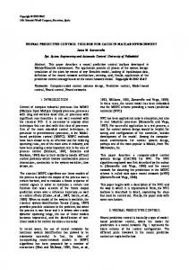
flotation column is a device used in the mineral industry to separate the valuable minerals from the carrier gangue. The column is fed with the ground ore and water, thus forming a slurry. Addition of air and adequate chemical reagents makes the valuable mineral particles rise at the top of the column, dividing it into two zones with different air holdups. The location of the interface between the zones is called the froth depth and is controlled by manipulating the reject flow rate at the bottom of the column. At the top of the column, a water stream washes out the entrained gangue particles from the mineralized bubbles, thus upgrading the concentrate recovered at the top. To ensure a downward flow of this wash water, a proper water balance must be kept in the upper zone of the column, otherwise the water added at the top might short-circuit to the concentrate without performing any cleaning action. This downward flow of water inside the upper zone is called the bias. The bias is controlled by manipulating the wash water flow rate. The control structure based on two monovariable GlobPC is illustrated in Figure 6. Decoupling in one direction is performed using the feedforward path of a GlobPC. Since the coupling in the second direction is weak, it is not taken into account. The performances of the system are shown in

27 Figure 7. Very good control was achieved by tuning the regulation and feedforward paths with a faster dynamics than the tracking modes.

The example illustrates that GloPC, because of its well decomposed structure, is very flexible (use of the feedforward path for decoupling), easy to implement (only 5 different objects) and to tune (all control modes are independent). Reference 29 also shows that nonlinearities can be handled with GlobPC by using a family of linear models.

7. CONCLUSION The key issue in GlobPC is to use three different controllers for tracking, disturbance rejection and feedforward, thus leading to perfect decoupling of all modes of control. A perfect separation between tracking and regulation dynamics was already available in PSMRC, while limited to onestep ahead setpoint tracking and long-range predictive regulation. GlobPC contains as a special case the GPC and UPC strategies which make use of a single objective function. The GlobPC structure, based on the internal model loop, cannot be implemented as such to control unstable processes. However, this structure exhibits many advantages, such as a clean separation of : • the tracking, regulation and feedforward dynamics, • the stochastic and deterministic predictions, • the stochastic and deterministic parts of the controllers, • the reference models for tracking, regulation and feedforward, • the partial state and complete model output,

28 Furthermore, the state-space representation simplifies the design of a single program for SISO and MIMO systems. All the well separated functions of the various parts of GlobPC make easier student training, control strategy design, computer object-programming and controller tuning. One unsolved drawback of GlobPC is the difficulty to handle constraints because of the presence of three objective functions.

8. ACKNOWLEDGMENTS The authors are grateful to the following funding organizations: CANMET (Canadian Centre for Mineral and Energy Technology), CRM (Centre de Recherche Minérale), FCAR (Fonds pour la Formation de Chercheurs et l’Aide à la Recherche), NSERC (Natural Science and Engineering Research Council of Canada) and a consortium of 14 Canadian mining and metallurgical companies.

9. REFERENCES

1. CUTLER, C.R. and RAMAKER, B.L.: 'Dynamic matrix control - A computer control algorithm', Proc. ACC, 1987, Minneapolis, USA.

2. DE KEYSER, R.M.C., VAN DE VELDE, G.A. and DUMORTIER F.A.G.: 'A comparative study of self-adaptive long-range predictive control methods', Automatica, 1988, 24(2), pp. 149-163.

3. YDSTIE B.E.: 'Extended horizon adaptive control', Proc. 9th IFAC World Congress, 1984, Budapest, Hungary.

29 4. CLARKE, D.W., MOHTADI, C. and TUFFS, P.S.: 'Generalized predictive control - Part I. The basic algorithm', Automatica, 1987, 23(2), pp. 137-148. 5. CLARKE, D.W., MOHTADI, C. and TUFFS, P.S.: 'Generalized predictive control - Part II. Extensions and interpretations', Automatica, 1987, 23(2), pp. 149-160.

6. RICHALET, J., RAULT, A., TESTUD, J.L. and PAPON, J.: 'Model predictive heuristic control: Applications to industrial processes', Automatica, 1978, 14(5), pp. 413-428.

7. M'’SAAD, M., DUQUE, M. and LANDAU, I.D.: 'Practical implications of recent results in robustness of adaptive control schemes', Proc. of the 25th CDC, December 1986, Athens, Greece, 1986.

8.. IRVING, E., FALINOWER, C.M. and FONTE: 'Adaptive generalized predictive control with multiple reference model', Proc. of the 2nd IFAC Workshop on Adapt. Syst. in Control and Signal Process., 1986, Lund, Sweden.

9. BORNARD, G. and GAUTHIER, J.P.: 'Commande multivariable des systèmes industriels de production', Internal note LAG #77-29, Laboratoire d'Automatique de Grenoble, November 1977.

10. FOULARD, C., GENTIL, S. and SANDRAZ, J.P. 'Commande et régulation par calculation numérique' (Ed. Eyrolles, Paris, 1987).

30 11. SOETERBOEK, A.R.M., VERBRUGGER, H.B., VAN DEN BOSCH, P.P.J. and BUTLER, H.: 'Adaptive predictive control - A unified approach', Proc. 6th Yale Workshop on Applic. of Adapt. Syst. Theory, 1990, New Haven, USA.

12. SOETERBOEK, A.R.M., VERBRUGGEN, H.B., VAN DEN BOSCH, P.P.J. and BUTLER, H.: 'On the unification of predictive control algorithms', Proc. 29th IEEE Conf. on Decision and Control, 1990, Honolulu, USA.

13. SOETERBOEK, R., 'Predictive Control : 'A Unified Approach' (Prentice Hall, Englewood Cliffs, 1992).

14. GARCIA, C.E. and MORARI, M.: 'Internal model control. 1. A unifying review and some new results', Ind. Eng. Chem. Process Des. Dev., 1982, 21(2), pp. 308-323.

15. MORARI, M. and ZAFIRIOU, E.: 'Robust Process Control' (Prentice Hall, Englewood Cliffs, 1989).

16. HODOUIN, D., GAGNON, É. and POMERLEAU A.: 'Autostop: A Unified Software for Simulation of Automatic Stochastic Optimal Control Loops', Proc. of 3rd Canadian Conf. on Computer Applications in the Mineral Industry, Montreal, Canada, 1995, pp. 796-805.

17. GOODWIN, G.C. and SIN, K.S. 'Adaptive Filtering, Prediction and Control' (Prentice Hall, Englewood Cliffs, 1984).

31 18. CLARKE D.W and GAWTHROP, P.J.: 'A self-tuning controller', IEE Proc. Control Theory Appl., 1975, 122(9), pp. 929-934.

19. BRUIJN, P.M., VERBRUGGER, H.B. and APPELDOORN, O.V.: 'Predictive control: A comparison and simple interpretation', Proc. IFAC Conf. on Low Cost Automation, 1986, Valencia, Spain.

20. ÅSTRÖM, K.J. and WITTENMARK, B.: 'On self-tuning regulators', Automatica, 1973, 9(2), pp. 185-199.

21. WELLSTEAD, P.E., PRAGER, D. and ZANKER, P.: 'Pole assignment self-tuning regulator', IEE Proc. Control Theory App., 1973, 126(8), pp. 781-787.

22. ÅSTRÖM, K.J. and WITTENMARK B.: 'Self-tuning controllers based on pole-zero placement', IEE Proc. Control Theory App., 1980, 127(3), pp. 120-130.

23. DESBIENS, A.: 'Commande distribuée algébrique et adaptative: Théorie, simulations et application industrielle', PhD Thesis, Department of Electrical and Computer Engineering, Université Laval, 1995.

24. LANDAU,.D.: 'Evolution of adaptive control', Trans. ASME, J. Dyn. Syst. Meas. Control, 1993, 115, pp. 381-391.

32 25. DESBIENS, A., NAJIM, K., POMERLEAU, A. and HODOUIN, D.: 'Adaptive control practical aspects and application to a grinding circuit', Optimal Control Appl. & Methods, 1996, 18, pp. 29-47.

26. M’SAAD, M. and SANCHEZ, G.: 'Multivariable generalized predictive control with a suitable tracking capability', J. Process Control, 1994, 4(1), pp. 45-52.

27. M'SAAD, M., LANDAU, I.D. and SAMAAN, M.: 'Further evaluation of for partial state reference adaptive design', Int. J. Adaptive Control and Signal Proc., 1990, 4, pp. 133-148.

28. DESBIENS, A., HODOUIN, D. and MILOT, M.: ‘Model-based predictive control: A general framework – Workshop on the observation, control and optimization of mineral processing and extractive metallurgy plants’, 38th Annual Conference of Metallurgist, 1999, Quebec City, Canada.

29. MILOT, M., DESBIENS, A., DEL VILLAR, R. and HODOUIN, D.: ‘Identification and multivariable nonlinear predictive control of a pilot flotation column’, XXI Int. Mineral Processing Congress, 2000, Rome, Italy.

33

Appendix A : Calculation of U'(t; t+HP-1) and ε(t+HS; t+HP) The trajectory of the future filtered control actions U'(t; t+HP - 1) is calculated by a repetitive application of the following state-space model derived from the transfer matrix Q(q-1) : X Q (t + 1) = AQ X Q (t ) + BQ u(t ) u' (t )

(A.1)

= CQ X Q (t ) + DQ u(t )

The vector U'(t; t+HP - 1) is : U' (t ;t + H P − 1) = NX Q (t ) + M' U (t;t + H P − 1)

(A.2)

with DQ   CQ   C B C A  Q Q   Q Q  2 N =  C Q AQ  M ' =  C Q AQ BQ    M   MP  H −1 HP− 2 C Q AQ BQ C Q AQ    

0 DQ CQ B Q M L

0  0 L L 0   DQ 0 L 0   M M M M L L L DQ   L

L

L

(A.3)

To express U'(t; t+HP - 1) as a function of U'(t; t+HC - 1), it is necessary to add the constraint S (q − 1 ) u(t + j ) = 0 for j ≥ H C

(A.4)

where S(q-1) is the following monic polynomial S(q − 1 ) = 1 − s1 q − 1 − s2 q − 2 − L − sns q − ns

Let us define Z(t) as the following vector of control actions :

(A.5)

34 u(t − ns + 1)  u(t − n + 2) s  Z (t ) =    K     u(t )

(A.6)

Then the constraint (A.4) can be written as follows

Z (t + H C ) = A Z (t + H C − 1) M Z (t + H P ) = A H

P

− H +1 C

(A.7)

Z (t + H C − 1)

where A is 0 0  A = 0  0 sn I  s

I

0

L

L

L

L

L

L

I

L

L

0

L

L

s2 I

0  L   0   I  s1 I  

(A.8)

with 0 and I being respectively zeros and identity matrices of order nu. Thus

where

with

U (t + H C ;t + H P − 1) = C Z (t + H C − 1)

(A.9)

 ßA   ßA 2   C =  L   H P -H C  ßA 

(A.10)

ß =[ 0 0 L

L

I]

(A.11)

35 and where 0 M  0  Z (t + H C − 1) = I 0  M 0 

0  M  K 0  0 K 0 U (t ; t + H C − 1) +  I M  O 0 K 0 I  K

I 0  0  0 0  M 0 

K 0  I M  O 0  K 0 I U (t + H C − nS ;t − 1) K 0  0 K 0  0

(A.12)

= VP U (t; t + H C − 1) + V S U (t + H C − nS ;t − 1)

If nS ≤HC , then U(t + HC – nS; t – 1) is zero. Finally,  U (t;t + H C − 1)  U (t;t + H − 1) =   C P U (t + H ;t + H − 1)    U (t;t + H C − 1) =  C C C V P U (t ; t + H − 1) + VS U (t + H − nS ;t − 1)  P

{

(A.13)

}

or

I 0 K 0 I  U (t ;t + H P − 1) = M O  0 K 0 C VP   = V1U (t ;t + H C

0  M  C 0 U (t ;t + H − 1) +  I   − 1) + V2U (t + H C −

0 K 0  M  M  U (t + H C − nS ;t − 1) 0 K 0   C VS   

(A.14)

nS ;t − 1)

Then (A.2) can be rewritten as a function of U(t; t+HC - 1) : U' (t ; t + H P − 1) = NX Q (t ) + Ω U (t ; t + H C − 1) + MU (t + H C − ns ; t − 1)

(A.15)

36 which is the Equation (7) with Ω = M' V1 and M = M' V2. The same calculation scheme applies to ε(t+HS; t+HP - 1), using the following state space form which embeds the process model G~ ( q − 1 ) and the filter F(q-1) :

X (t + 1) = AX (t ) + Bu(t ) + Cr (t ) e (t ) = DX (t ) + Er (t )

(A.16)

The future trajectory of the filtered deviation e(t+HS) to e(t+HP) is given by :

ε(t + H S ;t + H P ) = HX (t ) + θ'U (t;t + H P − 1) + LR(t;t + H P )

(A.17)

with  DA H  DA H − 1B  H S + 1  S DA DA H B    θ' = H=  M   M   HP−1 P  H B  DA   DA   S

DA H − 1C  L= M DA H P − 1C  S

S

DA H − 2 B L DAB HS −1 DA B L L M M M L L L S

DA H − 2C L DAC M M M L L L S

DB DAB M L

0 0 L   DB 0 L   M M  L L DB  (A.18)

DC E 0 L   M M M M L L L E 

Replacing into (A.17) U(t; t+HP-1) by its expression of (A.14), one obtains Equation (8)

ε(t + H S ;t + H P ) = HX (t ) + Θ U (t;t + H C − 1) + KU (t;t + H C − nS ;t − 1) + LR(t;t + H P ) (A.19) with Θ = θ'V1 K = θ'V2

(A.20)

37

Captions to illustrations Figure 1 : Process model. Figure 2 : Reference trajectories. Figure 3 : GlobPC structure. Figure 4 : Optimal controller CT, CF or CR. Figure 5 : GlobPC object-oriented programming. Figure 6 : Flotation column: Control structure. Figure 7 : Flotation column: Closed-loop trends.

38

u(t)

Gu(q-1)

ξ(t)

Gξ(q-1)

ζ (t)

Gζ (q-1)

Desbiens, Hodouin and Plamondon Figure 1

v(t)

yu(t) yξ(t)

+ +

Gv(q-1)

y(t) +

yv(t)

39

wT(t)

GT(q-1)

wR(t)

GR(q-1)

wF(t)

GF(q-1)

Desbiens, Hodouin and Plamondon Figure 2

rT (t) rR(t) +

+

+ rF (t)

rΣ(t)

40

P//-GF(q-1) Gv(q-1) Gζ (q-1)

rF (t)

wF(t)

RF (t + H ; t + H ) S F

P F

CF

ξ(t)

CT

+ RT (t + H TS ; t + H TP ) P//GT(q-1) SP

+

Gv(q-1) yv(t)

u (t) Process

+ uR(t)

Gu(q-1)

y(t) +

yu(t) -

yξ(t)

CR -1

-1

GT(q )

wR(t) RR (t + H ; t + H ) S R

P R

G R(q-1)

SP P//-GR(q-1) Gξ(q-1)

Desbiens, Hodouin and Plamondon Figure 3

-1

v(t)

rT (t)

wT(t)

ζ (t)

Gζ (q-1)

uF(t) uT(t)

G F(q-1)

rR(t)

41

F(q-1)

R(t+HS; t+HP)

+ ε(t+HS; t+HP) _

Q(q-1)

S(q-1)

Min J

Ex

W Λ HC HP HS ~ Y(t+HS; t+HP) U(t; t+HP+1) ~ G (q − 1 ) CT, CR or CF

Desbiens, Hodouin and Plamondon Figure 4

u(t)

42

Feedforward

v(t) ξ(t) Tracking

+

+

u(t)

y(t)

Process

+ -

wT(t)

Deterministic predictor

+ -

Regulation

Linear model

Desbiens, Hodouin and Plamondon Figure 5

Stochastic predictor

Controller

Sum

43

CR1

P//...

GR1

-1

uR1(t) w T1(t)

GT1

P//...

CT1

uT1(t)

u1(t)

+

+

CF1

GF1

-1

Reject flow rate Wash water flow rate

Process

uF1(t)

P//...

-

-

Gu1

Froth depth Bias

GV1 w T2(t)

GT2

P//...

CT2

uT2(t)

+

u2(t)

+

Gu2

-

GR2

-1

uR2(t)

CR2

Desbiens, Hodouin and Plamondon Figure 6

P//...

Froth depth(cm)

44

80 Measurement Setpoint

60 40 20 0

10

20

30

40

50

60

70

80

90

Bias(cm/s)

0.2 Measurement Setpoint 0.1 0

10

20

30

40

50

60

70

80

90

Control actions

1.5 Reject flow rate Wash water flow rate

1 0.5 0 0

10

20

Desbiens, Hodouin and Plamondon Figure 7

30

40 50 Time (min)

60

70

80

90