Global Vector Field Computation for Feedback Motion Planning Liangjun Zhang, Steven M. LaValle, and Dinesh Manocha http://gamma.cs.unc.edu/feedbackplanning Abstract— We present a global vector field computation algorithm in configuration spaces for smooth feedback motion planning. Our algorithm performs approximate cell decomposition in the configuration space and approximates the free space using rectanguloid cells. We compute a smooth local vector field for each cell in the free space and address the issue of the smooth composition of the local vector fields between the non-uniform adjacent cells. We show that the integral curve over the computed vector field is guaranteed to converge to the goal configuration, be collision-free, and maintain C ∞ smoothness. As compared to prior approaches, our algorithm works well on non-convex robots and obstacles. We demonstrate its performance on planar robots with 2 or 3 DOFs, articulated robots composed of 3 serial links and multi-robot systems with 6 DOFs.
I. INTRODUCTION Motion planning has been studied intensively in robotics [1], [2], [3]. Most of the earlier work focuses on computing collision-free paths in the robot’s free space which is the collision-free subset of its configuration space. In this paper, we address the problem of feedback motion planning, which deals with computing a feedback plan by computing a global vector field over the entire free space. Earlier work on decoupling the feedback and motion planning can be inefficient. Typically, paths computed by planners may not be smooth and can be difficult to track. On the other hand, it can be difficult to design feedback control strategies that take into account non-convex constraints induced by the obstacles in the environment. Therefore, when a feedback controller fails to steer the robot to follow a prescribed path, the robot often has to replan for a new path. In order to overcome these problems, feedback motion planning approaches take into account feedback concerns during collision-free path computation. Rather than planning a single collision-free path between the initial and goal configurations, these approaches compute a feedback plan over the entire free space of the robot that can converge towards the goal [4], [5]. A feedback plan is often represented as a vector field over the free space. Moreover, the resulting vector field satisfies the convergence property, i.e. the robot is guaranteed to arrive at the goal configuration without colliding with any obstacles in the environment. Most of the prior work on computing global vector fields for feedback motion planning is based on sequential composition [4], [5], [6], [7]. In these approaches, the robot’s free space is decomposed into cells. A local vector field This research is supported in part by ARO Contracts DAAD19-021-0390 and W911NF-04-1-0088, NSF awards 0400134, 0429583 and 0404088, DARPA/RDECOM Contract N61339-04-C-0043 and Intel. Steven M. LaValle is supported in part by NSF CISE grant number 0535007. Liangjun Zhang and Dinesh Manocha are with the Department of Computer Science, University of North Carolina, Chapel Hill, NC 27514, USA, {zlj,dm}@cs.unc.edu; Steven M. LaValle is with the Department of Computer Science, University of Illinois at Urbana-Champion, IL 61801, USA,
[email protected].
is computed within each cell and a global vector field is composed of individual vector fields. However, most prior algorithms are limited to low DOF robots and obstacles with simple shapes due to the difficulty of handling nonconvex collision constraints [7]. Other approaches assume that a good cell decomposition of the robot’s free space, e.g. the cylindrical algebraic decomposition (CAD), is given a priori [5]. Although CAD is an exact decomposition scheme and be used for general motion planning problems [8], it is difficult to implement this scheme robustly and efficiently, even for low DOF robots. As a result, most prior practical algorithms for feedback motion planning have been limited to simple robots with three or fewer DOFs. Main Results: In this paper, we present a practical global vector field computation algorithm for smooth feedback motion planning. Our algorithm performs approximate cell decomposition method that efficiently decomposes the robot’s free space into rectanguloid cells adaptively. We construct a smooth vector field within each cell in the free space and address the issue of smooth composition between the nonuniform adjacent cells. We also show any integral curve over the vector field is guaranteed to asymptotically converge to the goal configuration, to avoid collision with the obstacles, and to be smooth. In practice, our algorithm is relatively simple to implement and we demonstrate its performance on planar robots with 2 or 3 DOFs, articulated robots composed of 3 serial links, and multi-robot systems with 6 DOFs. Organization: The rest of the paper is organized as follows. In Section II, we briefly survey the related work. We formally define our problem in Section III and present the algorithm in Section IV. In Section V, we analyze some properties of the computed vector field and highlight the performance in Section VI. II. PREVIOUS WORK A. Motion Planning and C-Space Decomposition Motion planning is a fundamental problem in robotics. Prior works on motion planning include potential field [1], sample-based [2], [3] and cell decomposition methods. Our approach is closely related to the cell decomposition methods, which decompose the free space of the robot’s configuration space (C-space) into cells. Various decomposition schemes include triangulation for a point-shaped robot [9], cylindrical algebraic decomposition for general motion planning problem [8], star-shaped cell decomposition algorithm for low DOF robots [10]. Most practical cell decomposition planning algorithms perform approximate cell decomposition [1], [11], [12]. These algorithms decompose the robot’s configuration space into simple shapes, e.g. rectanguloid cells. The union of all cells in the free space is an approximation of the robot’s free space.
Free Space
Fig. 1. The robot’s configuration space is subdivided into cells. A discrete plan as a tree is computed over all cells in the free space.
B. Feedback Motion Planning Feedback motion planning generates a feedback plan over the entire free space for the robot to arrive at the goal. The feedback plan usually is represented as a vector field. One can also use potential field methods to compute navigation functions [13], [14], and further derive the vector fields by taking the gradients. The more direct approaches are to compute the vector field based on sequential composition [4], [5], [6]. By incorporating the non-holonomic and dynamic constraints, these approaches can compute vector fields for car-like robots [15]. Most of these approaches compute feedback plans with the convergence property. A quad-tree based decomposition has been used for feedback planning on a simple 2D robot with 2 translational DOFs and is further extended for 3D translational robots [7]. A feedback planning algorithm based randomized sampling is presented in [16]. Finally, the problem of designing global vector fields also arises in graphics, simulation and many other fields [17]. However, the underlying constraints are different. III. P ROBLEM D EFINITION In this paper, we consider a robot (or a multi-robot system) navigating in a static environment with non-convex obstacles. The configuration space C of each robot or multi-robot system is composed of the free space F and the configuration space obstacle (C-obstacle) O, where the exact boundary of C-obstacles is difficult to compute due to the underlying complexity. Given a goal configuration qgoal ∈ F, we need to compute a vector field V over the free space. For any configuration q in the same connected component in F as qgoal , the vector field V needs to satisfy the following properties: 1) its integral curve starting from q over the vector field V should converge to the goal configuration qgoal ; 2) its integral curve should lie completely in the free space; 3) its integral curve is smooth (e.g. C∞ differential). The implication of such a vector field is that for any free configuration in the same component as qgoal , there is always a collision-free path induced by the vector field. Therefore, such a vector field is a feedback plan for the given robot with the goal configuration qgoal . In the next section, we describe our algorithm to compute such a vector field over an approximation of the free space. IV. V ECTOR F IELD C OMPUTATION A LGORITHM In order to compute a vector field, we first perform approximate cell decomposition to subdivide the robot’s C-
space into cells. Given the decomposition, we compute a discrete plan which captures the global connectivity of the free space. We then construct a local vector field within each cell in F. Finally, a global vector field over the free space is the composition of the local vector field associated with each cell. A. Discrete Plan In order to capture the global connectivity of the free space F, we perform approximate cell decomposition (Fig. 1). The robot’s C-space is decomposed into rectanguloid cells (i.e. quad-tree decomposition for 2D C-space, octree decomposition for 3D C-space and so on). A cell is labelled as empty if it lies entirely in F, as full if it lies in O, and mixed otherwise. If a cell is mixed, the cell is further decomposed into smaller cells. One of the major issues with approximate cell decomposition is efficient labelling and classification of each cell. We use the cell labelling algorithm proposed by [12], [18], which is based on computing separation distances and penetration depths at different configurations of the robot with the obstacles. Overall, the approximate cell decomposition generates a set of empty cells, which provides an approximate representation of the robot’s free space F. A connectivity graph between the cells is extracted from the decomposition. Specifically, the connectivity graph G is defined where a node corresponds to an empty cell, and an edge denotes the adjacency between two empty cells in the decomposition. We compute a discrete plan based on the connectivity graph. For any empty cell, a discrete plan specifies its successor cell so that when recursively following the successor cell, the goal cell that consists of the goal configuration qgoal will be finally reached. In order to compute such a discrete plan, we first locate the node in the connectivity graph G corresponding to the goal cell. Beginning at this node, we perform the breadth first search (BFS) on the graph G and compute a tree that corresponds to that search. The tree represents a discrete plan and the cell for each node has only one successor cell (i.e. the parent node in the tree) except the goal cell, which can have multiple descendant cells (i.e. the children nodes in the tree). In our algorithm, the decomposition over C-space can be refined incrementally. Initially, the approximate cell decomposition computes a coarse approximation of the free space of the robot. If no path can be computed using the coarse approximation (e.g. the robot’s initial configuration lies in a mixed cell), we refine the decomposition. Specifically, we iteratively subdivide a fraction of all mixed cells identified by the first graph cut algorithm until a path connecting a robot’s initial configuration and goal configuration is computed or no such path exists for this problem [1], [12]. The discrete plan is computed based on the resulting decomposition. B. Vector Field Computation within Cells Based on the discrete plan described above, we compute a smooth vector field for each empty cell. If the cell is an intermediate cell in F (i.e. does not consist the goal configuration), the local vector field in C guides the robot
Face vector fields
C
f f1
Cell vector fields
f f1 C1
C
C1
virtual face
q
qm
fi Fig. 3. A GVD is defined for all faces (including the virtual faces) of a cell. For a configuration q, a influencing face fi is defined as the closest face of its cell.
(a)
(b)
Fig. 2. Choosing the appropriate face vector fields and cell vector fields for the two cases: uniform and non-uniform adjacent cells. f is a face in C and f1 is a face in C1 . We consider two different cases: Case (a), f ⊆ f1 and Case (b), f ⊃ f1 .
through the cell to its unique successor cell; if it is a goal cell, the vector field brings the robot to the goal configuration. We also desire that the vector field computed in each cell be smooth. In order to compute such a local vector field, we follow the general scheme described in [5]. For every face of the cell, we choose a face vector field Vf defined over the points on the face. We further choose a cell vector field Vc for points within the cell. The overall vector field V defined at any point p in the cell is a smooth interpolation of Vf and Vc . The different resolutions or sizes between adjacent cells pose a difficulty in terms of choosing the appropriate face or cell vector fields. Consider an intermediate cell C with its successor C1 (Fig. 2). In n dimensional C-space, each cell has 2n faces. Suppose the face f in C is sharing a boundary with the face f1 in C1 . We consider two different cases: Case (a): Fig. 2(a) shows this simpler case where the size of f is smaller than or equal to f1 (i.e. f ⊆ f1 ). Here the face f is defined as an exit face of the cell C since the vector field of C needs to cross the face to enter its successor C1 . Therefore, the face vector field Vf is chosen to be orthogonal to the face and points outwards. For other faces in C, their face vector fields are chosen to be orthogonal and point inwards. Finally, the cell vector field Vc is chosen to be identical to the face vector field of the exit face (Fig. 2(a)). Case (b): The other case is when f ⊃ f1 (Fig. 2(b)). In this case, the face vector field of f can not always point outwards. Otherwise, the vector field for the region f −f1 will not guide the robot to its successor cell C1 . To order to overcome this problem, a straightforward solution is to further subdivide the cells until the size of each cell becomes the same (i.e. a uniform subdivision of the entire free space). However, this can result in too many cells in the overall decomposition. Other approaches such as splitting the bigger cell so that f = f1 are difficult to be implemented for high dimensional space. Rather, we introduce the notion of a virtual face. As shown in Fig. 2(b), for the face f on C, over the region shared by both C and C1 , the face vector field is defined as pointing outwards and such a region is also referred to as an exit face. The rest of the region in f is covered by multiple virtual faces. Each virtual face has the same size as the exit face, and its face vector field is defined as pointing inwards.
Finally, the cell vector field Vc at a configuration q in the → , where qm cell C is chosen by normalizing the vector − qq m is the centroid point in the face f1 . It should be noted in our implementation, we don’t instantiate the virtual faces. Rather they can be interpreted indirectly from the adjacent cells to C. Next, we deal with the goal cell. There is no exit face for the goal cell. Therefore, every face vector field Vf can be chosen to be orthogonal to the face and point inwards. The cell vector field Vc (q) is chosen as the normalization of the → vector − qq goal . With the face vector fields Vf and the cell vector field Vc defined for all cells in the free space, we smoothly interpolate between them as [5] to compute the overall vector field in each cell. Given a configuration q in an intermediate cell, we first determine the closest face fi in this cell and define it as the influencing face. Therefore, all the faces of the cell determine a generalized Voronoi diagram of cell (GVD) as shown in Fig. 3. Now, V (q), the vector field at configuration q is defined as: (1) V (q) = norm((1 − b(q))Vfi (q⊥) + b(q)Vc (q)). Here q⊥ is the projection of q on the face fi . b(q) is a weighting function or bump function, whose value is 0 when q is on any face of the cell, and 1 on the GVD of the cell and interpolates between them according to the ratio of the distance to the influencing face and the other faces of the cell. In theory, any interpolation function that satisfies these conditions can be used. We use a C ∞ function presented in [5]. Moreover, in a goal cell, a subdivision is defined by considering the convex hull of the goal configuration qgoal and every face of the cell. The influence face then is computed based on the convex hull that the configuration q lies in. Finally, the global vector field over the entire free space from the decomposition is the composition of the vector field associated within each cell. V. A NALYSIS In this section, we analyze the properties of our vector field computation algorithm. Theorem 1: (Convergence) For any configuration q in the same connected component in F as qgoal , the integral curve starting from q over the computed vector field V asymptotically converges to qgoal . Building on the formulation shown in [5], we prove the convergence property by first showing that any integral curve over the vector field in an intermediate cell must reach its
(a)
(b)
(c)
(d)
(e)
(f)
Fig. 4. Gear Benchmark. (a) The problem is to compute a feedback plan for a 2-DOF translating gear-shaped robot in an environment with static obstacles. (b) The C-space is subdivided into cells adaptively. (c) A discrete plan is computed as a tree with the root highlighted as the black dot. (d) The vector field over the free space. The shaded regions denotes C-obstacles. For any collision-free configuration which is in the same component as the goal configuration, its integral curve converges to the goal. Any integral curve is smooth, though it may have high-variation in some region. (e) The zoom-in on the yellow region in (e) shows the integral curve is smooth. (f) The robot moves along an integral curve towards the goal.
exit face and proceed to its successor cell. Specifically, we prove the following two lemmas. Here, a GVD is defined for all faces of an intermediate cell C (Fig. 3). Lemma 1: Any integral curve cannot cross a GVD face of an intermediate cell C more than once. Proof: According to Eq. 1, V at any point q on a GVD face is equivalent to Vc (q). Therefore, for a GVD face with normal n, the sign of dot product between n and Vc (q) for any q on the face is fixed for both cases we have considered. Consequently, a GVD face cannot be crossed more than once. Lemma 2: Any integral curve in an intermediate cell C will reach its exit face. Proof: Denote the influencing face of q in C as fi . We determine the first GVD face f1 that intersects with the ray from the point q with the direction V (q). If there is no intersection, q is in the Voronoi region of the exit face and it is obvious that the integral will continue to the exit face. Otherwise, the signs of the dot products between the normal of f1 and the vectors Vc (q), and between this normal and Vfi will be the same. The overall vector field at q is a linear combination of Vc and Vfi . Therefore, on the integral curve, the distance to f1 is always decreasing. Consequently, either f1 or some other GVD face will be reached by the integral curve. Since there are a finite number of GVD faces in each intermediate cell and the integral curve cannot cross a GVD face more than once (Lemma 1), the integral curve finally will reach the exit face of the cell.
To complete the proof of the convergence property, we still need to show that the integral curve in a goal cell terminates at the goal configuration. For any point q, the distance to goal − → configuration qgoal is always decreasing since Vf · qq goal > − → > 0. Consequently, the dot product for its linear 0, Vc · qq goal combination of Vf and Vc is larger than 0. Collision-free Planning: Our integral curve is guaranteed to be collision-free, i.e. fully lie in the free space. This holds since in an intermediate cell, except for the exit face, the face vector field always points inwards and the weighting function for any point on the face is 0. Therefore, the only way an integral curve exits an intermediate cell is to cross through the exit face to its successor cell, which lies in the free space. In the goal cell, all the face vector fields point inwards. Therefore, the integral curve cannot exit from the goal cell. In conclusion, the integral curve fully lies in the free space and is guaranteed to be collision-free. Smoothness: Same as [5], our integral curve is also smooth or C ∞ differentiable. Within a cell, the vector field is smooth except on a set of measure zero (the d − 2 dimensional boundary of a cell; e.g. the vertices of a cell in 2D) since the chosen weighting function b for interpolating Vc and Vf is smooth. Furthermore, the vector field on the face between a cell and its successor is also smooth since all the derivatives of the weighting function on the boundary are 0. Therefore, the integral curve over V is smooth. Algorithm Complexity: The complexity of the overall algorithm is governed by the approximate cell decomposition
Fig. 6. 3-DOF Gear-shaped robot: The vector field guides the robot from its initial configurations towards the goal. Fig. 5. 3-DOF L-shaped robot: The computed vector field can guide the robot from any initial configuration to the goal.
# DOF tdec (s) level of subdivision # Cells Memory (MB) Per Point Loc.(μs) Per Evaluation(μs) Eva. Frequency:kHZ
Gear
Gear (3-DOF)
L-Shape
3-Link
Multi -Robot
2 3.01 11
3 10.5 6
3 9.84 6
3 186.2 5
6 23.97 3
46,510 38 1 13 78.9
133,512 242 2 26 38.2
182,288 304 2 24 41.1
72,262 190 2 47 21.2
297,424 451 2 61 16.3
TABLE I P ERFORMANCE OF O UR A LGORITHM ON DIFFERENT EXAMPLES .
step for computing the discrete plan. In the worst case, its complexity can increase exponentially with the number of DOFs. The local vector field computation algorithm within each cell has complexity of O(n) for determining the influencing face of a given configuration, where n is the number of faces (including the virtual faces) of the cell. Limitations: We discuss some limitations of our approach. Though the integral curves over the vector fields are guaranteed to be C ∞ smooth, the curves can sometimes have sharp turns due to the underlying adaptive decomposition. In the worst case, the number of cells increases exponentially as a function of the number of DOFs. Finally, in theory, no smooth vector field exists in a non-contractible free space. However, our vector field has additional non-smoothness on some boundaries of the cells: if the nodes in the discrete plan for two adjacent cells are not connected by an edge, the vector field along their common face is not smooth. To overcome this limitation, one may simplify the discrete plan. VI. R ESULTS We have implemented our vector field computation algorithm. We use an approximate cell decomposition method developed in [12] to subdivide the C-space. The implementation is general for arbitrary dimensional C-space. In our implementation we parameterize the rotation using Euler angles. During the decomposition, the angles are partitioned into intervals and are allowed to wrap around. The cell labelling to determine whether a cell lies entirely in free space or C-obstacle is performed by computing the separating distance or penetration depth computation between the
robot and obstacles [12]. We compute the discrete plan as a tree using the breadth first search. We choose the appropriate face vector field and cell vector field for the two cases as described in Section IV. In order to compute an integral curve, we use the Runge-Kutta integration method. We have tested our implementation on planar robots with 2-3 DOFs and multi-robot systems up to 6 DOFs. Fig. 4 shows a gear-shaped robot navigating in a 2D plane with 2 translational DOFs. We compute the vector field for the given goal configuration and highlight the integral curve for an initial configuration. The integral curve path is collisionfree and converges to the goal configuration. It should be noted the integral curve is indeed smooth, though the curve haves high variation in some regions. Fig. 5 shows an Lshaped robot navigating in a 2D environment. The robot has 3 DOFs and can both translate and rotate in the plane. We have applied our algorithm to articulated robots. Fig. 7 shows an example on an articulated robot composed of 3 serial links in a plane. The level of subdivision is 5, i.e in each dimension 25 decompositions are applied. Next, the first graph cut algorithm mentioned in Section IV is used to incrementally refine the decomposition. Finally, a global vector field is constructed and used to guide the robot to the goal. Due to the underlying axis-aligned decomposition, the robot sometimes moves one link a time. Fig. 8 shows an example of feedback planning for a multirobot system. The system is composed of three robots, and each robot has 2 translational DOFs. We compute a feedback plan for this system. This example may be difficult for a decoupled multi-robot planner. When moving towards its goal, each robot is blocked by other robots. Instead, we perform approximate cell decomposition on the composite 6D configuration space and compute vector fields on 6D cells in the free space. Given an initial configuration for the multi-robot system, we compute an integral curve over the global vector field. The motion for each robot is computed by projecting the 6D integral curve in a 2D plane. It should be noted that the integral curve in 6D is smooth. However, as shown in the figure, the motion for each robot may exhibit high variation or “cusps” due to the projection to a lower dimensional space.
Fig. 7. An articulated robot composed of 3 serial links. The vector field guides the robot to its goal qgoal .
Table I highlights the performance of our vector field computation algorithm. All the timings reported were generated on a 2.8GHz Pentium IV PC with 2 GB of memory. In the table, tdec denotes the total timing to perform the approximate cell decomposition, which is the major computationintensive step in our algorithm. The total number of cells and the memory usage are also reported for each example. Overall, our algorithm can efficiently compute vector fields for smooth feedback planning for these examples. We have also tested the performance on evaluating the constructed vector filed (shown in Table I). For each example, we randomly generate 1 million samples in the robot’s configuration space. Based on the approximate cell decomposition, we can efficiently locate the cell containing each sample in the logarithmic complexity. For any sample lying inside an empty cell, we evaluate its vector. Each evaluation takes only 13 − 61 microseconds in average; the corresponding frequency is 78.9 − 16.3 kHZ. VII. C ONCLUSION We present a practical global vector field computation algorithm in configuration space for smooth feedback motion planning. We perform approximate cell decomposition method over C-space and computer smooth vector field for each cell in the free space. We address the issue of smooth composition between non-uniform adjacent cells. We show that the integral curve over the computed vector field is guaranteed to converge to the goal configuration, avoid collision, and maintain C ∞ smoothness. As compared to prior work, our algorithm is practical for robot and obstacles with non-convex shapes and is simple to implement. We have demonstrated the performance of the algorithm on complex planar robots with 2 or 3 DOFs, articulated robots composed of 3 serial links and multi-robot system with 6 DOFs. There are several avenues for future work. We are interested in improving the quality of integral curves, e.g. reducing the high-variation on the curves. We are also interested in combining our feedback planning algorithm with randomized sampling techniques for higher DOF robots. Finally, we would like to extend our algorithm to robots with non-holonomic and dynamic constraints and apply the algorithm to crowd simulation [19]. R EFERENCES [1] J. Latombe, Robot Motion Planning. 1991.
Kluwer Academic Publishers,
Fig. 8. Feedback planning for a multi-robot system with 3 translating planar robots. [2] H. Choset, K. Lynch, S. Hutchinson, G. Kantor, W. Burgard, L. Kavraki, and S. Thrun, Principles of Robot Motion: Theory, Algorithms, and Implementations. MIT Press, 2005. [3] S. M. LaValle, Planning Algorithms. Cambridge University Press (also available at http://msl.cs.uiuc.edu/planning/), 2006. [4] D. C. Conner, A. A. Rizzi, and H. Choset, “Composition of local potential functions for global robot control and navigation,” in Proceedings IEEE/RSJ International Conference on Intelligent Robots and Systems, 2003, pp. 3546–3551. [5] S. R. Lindemann and S. M. LaValle, “Simple and efficient algorithms for computing smooth, collision-free feedback laws over given cell decompositions,” International Journal of Robotics Research, to appear, 2008, http://msl.cs.uiuc.edu/∼lavalle/papers/LinLav06c.pdf. [6] C. Belta, V. Isler, and G. J. Pappas, “Discrete abstractions for robot motion planning and control in polygonal environments,” IEEE Transactions on Robotics, vol. 21, no. 5, pp. 864–874, Oct. 2005. [7] M. Kloetzer and C. Belta, “A framework for automatic deployment of robots in 2d and 3d environments,” in Proceedings IEEE/RSJ International Conference on Intelligent Robots and Systems, 2006, pp. 953–958. [8] J. T. Schwartz and M. Sharir, “On the “piano movers” problem I: The case of a two-dimensional rigid polygonal body moving amidst polygonal barriers,” Commun. Pure Appl. Math., vol. 36, pp. 345–398, 1983. [9] A. Narkhede and D. Manocha, “Fast polygon triangulation based on seidel’s algorithm,” in Graphics Gems V, A. Paeth, Ed. New York: Academic, 1995, pp. 394–397. [10] G. Varadhan and D. Manocha, “Star-shaped roadmaps - a deterministic sampling approach for complete motion planning,” in Proceedings of Robotics: Science and Systems, Cambridge, USA, June 2005. [11] R. Brooks and T. Lozano-P´erez, “A subdivision algorithm in configuration space for findpath with rotation,” in Proc. 8th Internat. Joint Conf. Artif. Intell., Aug. 1983. [12] L. Zhang, Y. Kim, and D.Manocha, “Efficient cell labelling and path non-existence computation using c-obstacle query,” The International Journal of Robotics Research, vol. 27, no. 11-12, pp. 1246–1257, NovDec 2008. [13] E. Rimon and D. E. Koditschek, “Exact robot navigation using artificial potential fields,” IEEE Transactions on Robotics and Automation, vol. 8, no. 5, pp. 501–518, Oct. 1992. [14] S. M. LaValle and P. Konkimalla, “Algorithms for computing numerical optimal feedback motion strategies,” International Journal of Robotics Research, vol. 20, no. 9, pp. 729–752, Sept. 2001. [15] S. R. Lindemann and S. M. LaValle, “Smooth feedback for car-like vehicles in polygonal environments,” in IEEE International Conference on Robotics & Automation, 2007, pp. 3104–3109. [16] L. Yang and S. M. LaValle, “The sampling-based neighborhood graph: A framework for planning and executing feedback motion strategies,” IEEE Transactions on Robotics and Automation, vol. 20, no. 3, pp. 419–432, 2004. [17] E. Zhang, K. Mischaikow, and G. Turk, “Vector field design on surfaces,” ACM Transactions on Graphics, vol. 25, no. 4, pp. 1294– 13 268, 2006. [18] L. Zhang, Y. Kim, G. Varadhan, and D.Manocha, “Generalized penetration depth computation,” Computer-Aided Design, vol. 39, no. 8, pp. 625–638, August 2007. [19] S. Patil, J. Berg, S. Curtis, M. Lin, and D. Manocha, “Directing crowd simulations using navigation fields,” Computer Science, UNC, Tech. Rep., 2009.