GPU accelerated lattice Boltzmann simulation for rotational turbulence

Author's personal copy Computers and Mathematics with Applications 67 (2014) 445–451

Contents lists available at ScienceDirect

Computers and Mathematics with Applications journal homepage: www.elsevier.com/locate/camwa

GPU accelerated lattice Boltzmann simulation for rotational turbulence Huidan (Whitney) Yu a,b,∗ , Rou Chen c , Hengjie Wang d , Zhi Yuan e , Ye Zhao e , Yiran An d , Yousheng Xu f , Luoding Zhu g a

Department of Mechanical Engineering, Indiana University Purdue-University Indianapolis, IN 46202, USA

b

College of Metrology & Measurement Engineering, Zhongguo Jiliang University, Hangzhou, China

c

Department of Physics, Zhejiang Normal University, Jinhua 321004, China

d

Department of Mechanics, College of Engineering, Peking University, Beijing, 100871, China

e

Department of Computer Science, Kent State University, OH 44242, USA

f

School of Light Industry, Zhejiang University of Science and Technology, Hangzhou 310023, China

g

Department of Mathematical Sciences, Indiana University Purdue-University Indianapolis, IN 46202, USA

article

info

Keywords: Rotation turbulence Turbulence scaling Lattice Boltzmann method GPU computing

abstract In this work, we numerically study decaying isotropic turbulence in periodic cubes with frame rotation using the lattice Boltzmann method (LBM) and present the results of rotation effects on turbulence. The implementation of LBM is on a GPU (Graphic Processing Unit) platform using CUDA (Compute Unified Device Architecture). Through the accelerated GPU-LBM simulation, we look into various effects of frame rotation on turbulence. It has been observed that rotation slows down the decay of kinetic energy and enstrophy. Rotation also breaks isotropy and induces vortex tubes in the direction of frame rotation. Characteristics related to velocity and its derivatives have been studied with and without rotation. Without rotation, the kinetic energy and enstrophy decay follow −10/7 and −17/7 scaling respectively whereas in the presence of rotation with the relatively small Rossby number (large rotation intensity), the energy decay slows down to −5/21 scaling when the initial isotropic turbulence energy spectrum is scaled to k4 . These scalings with and without rotation are in quantitative agreements with the predictions from Kolmogorov hypotheses respectively. The skewness and kurtosis are seen more fluctuating in rotational turbulence, which agrees with the results from NS-based computation. Using this accelerated and validated GPU-LBM computation tool, we are further studying the inverse energy transfer behavior with and without rotation aiming to quantify the effects of rotation on the inverse energy transfer to reveal underlying physics of a particular stage of the turbulence development. The results will be presented in near future. Published by Elsevier Ltd

1. Introduction Decaying isotropic turbulence (DIT) in a periodic box has enabled much of our progress in understanding universal features of turbulence. Although artificial, isotropic turbulence defies much beyond the well-known Kolmogorov k−5/3 energy spectrum [1] in the inertial range where k is the wave number. When the box is subjected to a rotation, e.g., for

∗

Corresponding author at: Department of Mechanical Engineering, Indiana University Purdue-University Indianapolis, IN 46202, USA. E-mail addresses: [email protected], [email protected] (H. Yu).

0898-1221/$ – see front matter. Published by Elsevier Ltd http://dx.doi.org/10.1016/j.camwa.2013.09.017

Author's personal copy 446

H. Yu et al. / Computers and Mathematics with Applications 67 (2014) 445–451

a vertical axis ( = Ωz k), the nonlinear flow dynamics will be modified. Whereas DIT in a non-rotating system remains approximately isotropic, the vertical length scale increases dramatically in the rotating case. In rotational turbulence, there exist two major time scales. One is τL ∼ L/urms associated with the eddies at characteristic integral length scale L and velocity urms . Another is τΩ ∼ 1/Ωz associated with rotation. These two time scales are characterized by √ the Taylor microscale Reynolds number (Reλ = urms λ/ν ) and the Rossby number (Ro = urms /(2Ωz L)), where urms = 2k/3 is the root mean square of velocity field, λ = 15ν u2rms is the transverse Taylor-microscale length, k is the kinetic energy, and ν is the kinematic viscosity of the fluid. The dynamics of rotational turbulence is dictated by a competition between the linear rotation effect and nonlinear turbulent energy transfer. Rotational turbulence is of significant importance in engineering, geophysical, and astrophysical flows. Efforts have been made to study the effect of rotation in a turbulent flow, as a first step to gain better understanding of the fluid dynamics of geophysical systems. Rotation plays an important role in such systems. For rapid rotation (very small Rossby numbers), significant progress has been made by applying resonant wave theory [2,3], two-point spectral closures [4,5], and weak turbulence theory [6]. In these approaches, the flow is considered as a superposition of inertial waves with a short period, and the evolution of the system for long times is derived considering the effect of resonant triad interactions. Recently, due to the development of computation capability, direct numerical simulation (DNS) and large-eddy simulation (LES), which solve the Navier–Stokes (NS), were performed [7,8] to study the effects of rotation on turbulence with a moderately small Ro number. In the last two decades, the lattice Boltzmann method (LBM) [9,10] has emerged as an alternative to solve fluid dynamics on the mesoscopic level for complex flows [11,12]. As opposed to conventional CFD which solves the NS equations directly, the LBM is based on the Boltzmann equation and kinetic theory [13]. One of the most attractive advantages of LBM over NS solvers is the suitability of parallelism due to its inherent local data access pattern. Recently, parallel computation on graphics processing units (GPUs) for scientific research emerged due to the high performance and efficiency of computation against the traditional computation on central processing units (CPUs). The computation capacity of GPUs is almost one order of magnitude larger than that of mainstream CPUs in terms of both peak performance and memory bandwidth. As a result, GPU parallel computation is promising to make the demanding computation tasks such as those in computational fluid dynamics [14,15] especially when the flow is turbulent. In LBM, the computation on each node is independent and the data transmission only happens between two adjacent nodes. This localized data communication mode and inherent additivity of its numerical implementation make LBM ideally suitable for GPU parallel computation. In the last few years, implementations of LBM on a single GPU have been reported [16–24] speedup ratios ranging from one to two orders of magnitude depending on the algorithms, the complexity of flows, and the hardware availability. Tölke et al. [20] used shared memory to avoid misaligned accesses at the expense of adding an extra kernel to exchange data on some nodes. On the latest GPUs, the performance of misaligned memory accesses is enhanced due to the improved hardware architecture. Obrecht et al. [24] used standard memory access and only one kernel in LBM simulation. The performance for D2Q9 model [24] was compared with Tölke’s shared memory scheme [20], showing a 15% improvement. The present work is part of our continuous efforts to investigate the universal features of DIT with and without rotation. In our previous work [25], we assessed the reliability of LBM for performing DNS and LES of DIT with and without frame rotation. Focuses were on the quantitative comparisons of decay exponents of the kinetic energy k, the dissipation rate ε , and the low wave-number scaling of the energy spectrum with established classical results. The LBM-LES captured the prominent large-scale flow behavior through the comparisons of LBM-DNS vs. LBM-LES and LBM-LES vs. NS-LES. It was concluded that both LBM-DNS and LBM-LES could well capture the important features of DIT. Due to the computation capability, the Taylor-microscale–Reynolds number, Reλ , was relatively low with maximum resolution of 1283 and the results for DIT in the presence of frame rotation was limited. In order to accelerate the computation to meet the demanding computation cost for turbulence and make it possible to perform computation on a local workstation, we implement LBM-DNS on the GPU platform based on the two existing schemes in open Refs. [24,20] and select the better one [24] to perform the simulation. We study various rotation effects on DIT with higher Reλ and smaller Ro. Our focus is on how rotation affects turbulence properties, such as the decay of the kinetic energy, dissipation rate, and vorticity, the development of energy spectrum, the evolution of velocity-derivative skewness and kurtosis, etc., which are keys on the turbulence energy cascade. The remainder of the paper is organized as follows: in Sections 2 and 3, we introduce lattice Boltzmann equations for DNS of rotational turbulence and the implementation of GPU parallel computing using CUDA. In Section 4, we present the results of rotation effects on turbulence. Finally Section 5 provides a summary discussion and concludes the paper. 2. Lattice Boltzmann method for rotational turbulence The LBM is based on grid computing which calculates the macroscopic physical quantities by mesoscopic particle interactions [26]. The lattice Boltzmann equation (LBE) deals with the time evolution of particle distribution fα (x + eα δt , t + δt ) = fα (x, t ) −

1

τ

[fα − fα(eq) ] + Fα

(1)

where fα is the single-partial distribution with discrete velocity eα and τ is the relaxation time caused by molecular collision. In this work, we use the 3D 19-velocity (D3Q19) model due to its reliability and efficiency of computation [27].

Author's personal copy H. Yu et al. / Computers and Mathematics with Applications 67 (2014) 445–451

447

Correspondingly, the discrete velocity sets are (0, 0) for α = 0; (±1, 0, 0)c , (0, ±1, 0)c , (0, 0, ±1)c for α = 1 ∼ 6; and (±1, ±1, 0)c , (0, ±1, ±1)c , (±1, 0, ±1)c for α = 7 ∼ 18. Parameter c is the lattice velocity defined as c = δ x/δt with δ x being the lattice length and δt the time step. In practice, c is usually set to 1. The equilibrium distribution function fα(eq) is formulated as [28] fα(eq)



= ωα δρ + ρ0



3eα · u c2

+

4.5(eα · u)2 c4

− 1.5

u2

 (2)

c2

where ωα is the weight coefficient, in D3Q19, ω0 = 1/3, ω1−6 = 1/18, ω7−18 = 1/36. The density ρ = ρ0 + δρ including the mean density in the system ρ0 and the fluctuation of density δρ and the macroscopic velocity are obtained by

δρ =

 α

fα =

 α

fα(eq) ,

ρ0 u =

 α

eα fα =

 α

eα fα(eq) .

(3)

The force term Fα is the discrete format of an external force [29] as Fα = −3ωα ρ0

eα · a c2

δt

(4)

where a is acceleration determined by the external force. In the rotating flow, a = −2z × u is the Coriolis force, where  is the angular velocity of the frame of reference acting in the z-direction,  = Ωz k. Through the Chapman–Enskog expansion [30], the LBE recovers Navier–Stokes equations as follows:

∂ρ + ρ0 ∇ · u = 0 ∂t ∂u + u · ∇ u = −∇ p + υ∇ 2 u + a ∂t

(5) (6)

√

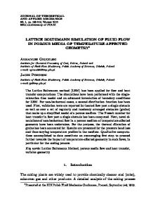
where p is the pressure which is given as p = cs2 ρ/ρ0 , cs is the sound speed of the model which is equal to c / 3, υ is the viscosity which is shown on the model as lattice units like υ = cs2 (τ − 1/2). 3. GPU parallel implementation The computation is carried out in a periodic cube with a size of Nx × Ny × Nz on the CUDA platform. Initially, an isotropic turbulence with prescribed energy spectrum [25] is injected in the cube and then the turbulence decays freely. In LBM, there exist four computation segments in each time step including collision, boundary condition, streaming, and velocity/density update. In CUDA, a block refers to a batch of threads that can cooperate via shared memory and have synchronized execution, whereas a warp is a group of threads as the minimal element processed in multiprocessors. We chose one dimensional block such that each warp can be aligned to the array. The size of a warp is 32 threads for all existing CUDA GPUs, yet this value might change with future hardware. The streaming, collision, and update of velocity and density are combined into one kernel to reduce access latency. Although this combination may cost more storage and lead to lower occupancy, it avoids repeated access of global memory for distribution functions and increases the efficiency of data communication. The distribution functions containing z component, which are f5 , f6 , and f11 − f18 in the D3Q19 lattice model, would have a shift along the z-axis. During the streaming, this misalignment would result in a misaligned access because the elements in our array starts from the z-axis. To address this issue, Tölke et al. [20] split the misaligned streaming into two parts, first to shift the data of distribution functions along the z-axis in shared memory and second to use aligned write to finish streaming. The shift requires a set of arrays with the size of (the number of threads per block) × (word size) to be allocated in the shared memory. For the D3Q19 lattice model, 10 arrays are needed. This amount usage of shared memory may limit the occupancy for some device. Tölke’s algorithm for the streaming segment is shown in Fig. 1(a). Obrecht et al. [24] proposed another approach based on two points. First, misaligned read is faster than misaligned write. Second, the additional kernel to exchange the data may consume more time than the misaligned access. As a result, instead of taking advantages of shared memory, they use misaligned read to carry on the streaming segment. After computation, all the data are written aligned to global memory; see Fig. 1. The CUDA implementation is on two Intel Xeon E5645 2.40 GHz Quad-Core CPUs and 64 GB memory with a Tesla M2090 GPU card with ECC enabled by default. Commonly, the performance of a GPU-LBM program is measured by millions lattice updated per second (MLUPS), which directly reflects how long it takes to finish the collision and streaming processes for all the nodes at one time step. Without considering rotation in this part, we list the MLUPS performance of the two schemes from [20,24] with single precision for four resolutions in Table 1. For the scheme using shared memory [20], Bailey [22] has claimed an average performance of 246 MLUPS with a maximum value of 300 MLUPS in the case of Poiseuille flow. For the scheme using misaligned read, Obrecht [24] tested for lid driven cavity flow and achieved a highest performance of 516 MLUPS. Our evaluation shows the highest performance of 460 MLUPS using misaligned read and 445 MLUPS using sheared memory scheme. The average performance of the former is around 455 MLUPS, and the latter around 430 MLUPS.

Author's personal copy 448

H. Yu et al. / Computers and Mathematics with Applications 67 (2014) 445–451

Fig. 1. (a) Shared memory scheme [20]. (b) Misaligned read scheme [24]. Table 1 Performances of misaligned [24] and shared memory [20] algorithm. Algorithm with misaligned read

Scale MLUPS

643 451

1283 460

1923 460

2563 449

Algorithm with shared memory

Scale MLUPS

643 438

1283 445

1923 381

2563 423

Table 2 GPU acceleration test comparing GPU-LBM and serial-CPU-LBM. The numbers in the ‘‘GPU’’ and ‘‘serial-CPU’’ columns are wall-clock time in second for 200 steps running. The speedup is measured as the ratio of time spent with and without GPU implementation. Resolution 3

64 1283 2563

GPU-LBM

Non-GPU-LBM

Speedup

1.0 13.57 190.1

235.32 3538.17 62 751.3

235.3 261.0 330.1

The misaligned method provides better performance on GPU acceleration. This shows that the straightforward misaligned memory access can satisfy the requirement of LBM-based turbulence acceleration. The shared memory approach may involve more processing efforts and no longer needed due to the improved GPU architecture. The preliminary test of computation speed shows outstanding acceleration of the developed GPU-LBM over the original serial CPU LBM. The comparison results are shown in Table 2. For the resolutions 1283 and 2563 which we use to study turbulence fundamentals, more than 250 times speed-up are achieved, which greatly increases our research efficiency since we are able to run 2563 case on our group workstation with fairly short computation duration. It should be pointed out that both the CPU and GPU based implementations are not extensively optimized by fully exploiting functionalities provided by the underlying hardware. In this paper, our focus is to present the underlying physics of rotational turbulence. We only show that the LBM simulation can be greatly accelerated by GPU acceleration, which makes it possible to perform the simulation of 2563 case on a local workstation. In the future, we will perform a thorough optimization of GPU programs and measure and analyze GPU performance in more detail and accuracy, and eventually lead to a public available platform for researchers.

4. Results of rotational turbulence We now present physical results for DIT in the presence of rotation using the developed GPU-LBM code based on Obrecht’s misaligned implementation [24]. All the results shown below are from 1283 and 2563 simulations. The initial energy spectra are scaled as k4 [25] unless otherwise indicated. We first show the decay of kinetic energy (E (t )/E0 ) and enstrophy (Ω (t )/Ω0 ) with no rotation (Ωz = 0) and energy decay with varying Ro numbers in Fig. 2. In the unbounded flows, in the case of an initial large scale spectrum ∼ k4 , theoretical predictions of the decay scalings of kinetic energy [31] and enstrophy [8] are E (t ) ∼ t −10/7 ,

Ω (t ) ∼ t −17/7 .

(7)

The LBM results in Fig. 2(a) quantitatively capture both scalings of −10/7 and −17/7 and are in quantitative agreement with established numerical results [8]. In Fig. 2(b), it is seen that the energy decay slows down when the Ro number decreases

Author's personal copy H. Yu et al. / Computers and Mathematics with Applications 67 (2014) 445–451

449

Fig. 2. Decay of energy and enstrophy. (a) Re = 95, 1283 , without rotation and (b) Re = 105, 2563 , with and without rotation.

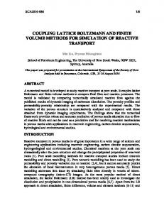
Fig. 3. Contours of ωz in late time originated from the same prescribed isotropic turbulence field (a) with Reλ = 95 in a 1283 . (b) without rotation (Ro = ∞) and (c) with rotation (Ro = 3).

corresponding to the increase of rotation from bottom up, indicating that rotation prohibits energy decay. When the rotation is strong enough, the energy decay is scaled as −5/21, agreeing with the Kolmogorov prediction [8]. The evolutions of z component of the vorticity (ω = ∇ × u) in 3D both in the condition of no rotation (b) (Ro = ∞) and with rotation (c) (Ro = 3) are shown in Fig. 3, both of which are originated from the same isotropic turbulence. Visualization of the flow vorticity is intuitive to read. It is clearly shown that without rotation, seen in Fig. 3(b), the vorticity field maintains isotropic at the late time, whereas with reference rotation, anisotropic behavior is observed. In Fig. 3(c), rotation induced vorticity tube in the z direction appears, implying the rotation effect on turbulence decay. This behavior was observed by Teitelbaum and Mininni [8] in their computation.

Author's personal copy 450

H. Yu et al. / Computers and Mathematics with Applications 67 (2014) 445–451

Fig. 4. Evolution of velocity-derivative skewness and kurtosis in the cases of (a) no rotation (Ro = ∞) and (b) rotation (Ro = 3), Reλ = 95, 1283 .

The velocity derivation characteristics are presented by skewness Si and kurtosis Ki defined as [8]

 Si =

 Ki =

∂ ui ∂ xi

3  

∂ ui ∂ xi

4  

∂ ui ∂ xi

2 3/2

∂ ui ∂ xi

2 2

(8)

(9)

respectively, where i presents the Cartesian coordinates x, y, and z. The results are presented in Fig. 4. It is shown that skewness and kurtosis in the case of no rotation, three components have no obvious fluctuation in Fig. 4(a). When the rotation is added, the consequence is shown in Fig. 4(b). It is seen that the three components of skewness and kurtosis have more fluctuation, while Sx ≈ −Sy , Kx ≈ Ky all the time. This result qualitatively agrees with what is presented in [8]. 5. Summary We have developed a GPU-LBM code using CUDA for simulating DIT in a periodic cube with and without frame rotation. The GPU parallel implementation has greatly accelerated the computation, around 300 times faster over non-GPU parallel, which makes it possible to run 2563 with Reλ approximately 120 on a local workstation with short computation duration. We run a large number of cases to systematically study various effects of rotation on turbulence. It has been showed that in the presence of rotation, energy decay slows down when the Ro number decreases, i.e., rotation increases. This indicates that rotation prohibits energy decay. The rotation induced vortex tube along the rotation axis is captured. The decay scalings of kinetic energy with and without rotation and the scaling of enstrophy quantitatively agree with the Kolmogorov analytical prediction, demonstrating that the developed GPU-LBM simulation is a reliable numerical tool to study underlying physics of rotational turbulence. In this study, we have observed that kinetic energy is not only transferred to small motion scales following the wellknown −5/3 Kolmogorov scaling, but also to a large motion, which is in the inverse direction of the well defined energy cascade (not shown here) before energy starts to decay. Using this accelerated and validated GPU-LBM computation tool, we parametrically investigate the scalings of inverse energy transfer and the rotation effects on the inverse energy transfer aiming to find universal features of the particular stage of the turbulence development. Meanwhile, we are implementing GPU-LBM on multiple GPU cards to further promote the computation efficiency. Acknowledgments The third author thanks Dr. Peng Wang, the Manager of HPC Developer Technology, NVIDIA China, for all the valuable advice and guidance on CUDA programming. This work was supported by the National Nature Science Foundation of China under Grant Nos. 10972208 and 11172219 and the International Development Fund (IDF) Grant from the Office of the Vice Chancellor for Research (OVCR) of Indiana University-Purdue University Indianapolis. References [1] [2] [3] [4]

S.B. Pope, Turbulent Flows, Cambridge University Press, Cambridge, 2000. H.P. Greenspan, The Theory of Rotating Fluids, Cambridge University Press, Cambridge, 1968. F. Waleffe, Inertial transfers in the helical decomposition, Physics of Fluids A (Fluid Dynamics) 5 (1993) 677. C. Cambon, L. Jacquin, Spectral approach to non-isotropic turbulence subjected to rotation, Journal of Fluid Mechanics 202 (1989) 295.

Author's personal copy H. Yu et al. / Computers and Mathematics with Applications 67 (2014) 445–451

451

[5] C. Cambon, N.N. Mansour, F.S. Godeferd, Energy transfer in rotating turbulence, Journal of Fluid Mechanics 337 (1997) 303. [6] S. Galtier, Weak inertial-wave turbulence theory, Physical Review E 68 (2003) 015301. [7] P.D. Mininni, A. Alexakis, A. Pouquet, Scale interactions and scaling laws in rotating flows at moderate Rossby numbers and large Reynolds numbers, Physics of Fluids 21 (2009) 015108. [8] T. Teitelbaum, P.D. Mininni, The decay of turbulence in rotating flows, Physics of Fluids 21 (2011) 065105. [9] Y. Qian, D. d’Humiéres, P. Lallemand, Lattice BGK models for Navier–Stokes equation, Europhysics Letters 17 (6) (1992) 479–484. [10] H. Chen, S. Chen, W. Mattheus, Recovery of the Navier–Stokes equations through a lattice gas Boltzmann equation method, Physical Review A 45 (1992) 5339–5342. [11] S. Chen, G.D. Doolen, Lattice Boltzmann method for fluid flows, Annual Review of Fluid Mechanics 30 (1998) 329–364. [12] C.K. Aidun, J.R. Clausen, Lattice-Boltzmann Method for Complex Flows, Annual Review of Fluid Mechanics 42 (2010) 439–472. [13] X. He, L. Luo, Theory of the lattice Boltzmann method: from the Boltzmann equation to the lattice Boltzmann equation, Physical Review E 56 (1997) 6811–6817. [14] J. Dongarra, G. Peterson, S. Tomov, Exploring new architectures in accelerating CFD for air force applications, in: Proceedings of HPCMP Users Froup Conference, 2008, pp. 14–17. [15] I.C. Kampolis, X.S. Trompoukis, V.G. Asouti, K.C. Giannakoglou, CFD-based analysis and two-level aerodynamics optimization on graphics processing units, Computer Methods in Applied Mechanics and Engineering 199 (2010) 712–722. [16] J. Tölke, M. Krafczyk, TeraFLOP computing on a desktop PC with GPUs for 3D CFD, International Journal of Computational Fluid Dynamics 22 (7) (2008) 443–456. [17] W. Ge, F. Chen, F. Meng, et al., Multi-Scale Discrete Simulation Parallel Computing Based on GPU, Science Press, Beijing, 2009 (in Chinese). [18] M. Bernaschi, M. Fatica, S. Mecchionna, S. Succi, E. Kaxiras, A flexible high-performance lattice Boltzmann GPU code for simulations of fluid flows in complex geometries, Concurrency and Computation: Practice and Experience 22 (2010) 1–14. [19] F. Kuznik, C. Obrecht, R.G. Rusaouën, J.J. Roux, LBM based flow simulation using GPU computing processor, Computers and Mathematics with Applications 59 (2010) 2380–2392. [20] J. Tölke, Implementation of a lattice Boltzmann kernel using the compute unified device architecture developed by NVIDIA, Computing and Visualization in Science (2008) 1–11. [21] J. Habich, Performance evaluation of numeric compute kernels on NVIDIA GPUs, Master’s Thesis, 2008, University of Erlangen-Nurnberg. [22] P. Bailey, J. Myre, S.D.C. Walsh, D.J. Lilja, M.O. Saar, Accelerating lattice Boltzmann fluid flow simulations using graphics processors, 2009. [23] A. Kaufman, Z. Fan, K. Petkov, Implementing the lattice Boltzmann model on commodity graphics hardware, Journal of Statistical Mechanics: Theory and Experiment (2009) P0601. [24] C. Obrecht, F. Kuznik, B. Tourancheau, J.J. Roux, A new approach to the lattice Boltzmann method for graphics processing units, Computers and Mathematics with Applications 61 (12) (2011) 3628–3638. [25] H. Yu, S.S. Girimaji, L. Luo, Lattice Boltzmann simulations of decaying homogeneous isotropic turbulence, Physical Review E 71 (2005) 016708. [26] D.A. Wolf-Gladrow, Lattice-Gas Cellular Automata and Lattice Boltzmann Models: An Introduction, first ed., Springer-Verlag, 2000. [27] R. Mei, W. Shyy, D. Yu, L. Luo, Lattice Boltzmann method for 3-D flows with curved boundary, Journal of Computational Physics 161 (2000) 680–699. [28] X. He, L. Luo, Lattice Boltzmann model for the incompressible Navier–Stokes equation, Journal of Statistical Physics 88 (1997) 927–944. [29] L. Luo, Theory of the lattice Boltzmann method: Lattice Boltzmann models for nonideal gases, Physical Review E 62 (2000) 4982–4996. [30] Z. Guo, T.S. Zhao, Lattice Boltzmann model for incompressible flows through porous media, Physical Review E 66 (2002) 036304. [31] T. Ishida, P.A. Davidson, Y. Kaneda, On the decay of isotropic turbulence, Journal of Fluid Mechanics 564 (2006) 455–475.