GPU processing for parallel image processing and real-time object ...

GPU processing for parallel image processing and real-time object recognition a

Kevin Vincentb, Damien Nguyenc, Brian Walkerd, Thomas Lua1, and Tien-Hsin Chaoa Jet Propulsion Lab/Caltech, Pasadena, CA, USA; bCalifornia State University, Fullerton; c Saddleback College; dGeorgia Inst. of Tech. Atlanta, GA, USA; ABSTRACT

In this paper, we present a method for reducing the computation time of Automated Target Recognition (ATR) algorithms through the utilization of the parallel computation on Graphics Processing Units (GPUs). A selected multi-stage ATR algorithm is refounded to encourage efficient execution on the GPU. Such refounding includes parallel reimplementations of optical correlation, Feature Extraction, Classification and Correlation using NVIDIA's CUDA programming model. This method is shown to significantly reduce computation time of the selected ATR algorithms allowing the potential for further complexity and real-time applications.

Keywords: automated target recognition, GPU, CUDA programming, parallelization, real-time, computer vision, optimization.

1. INTRODUCTION

Automated Target Recognition (ATR) is an area of computer vision wherein a machine extracts useable information from image data. Such information could include the presence, or absence, of the target objects along with their relative location from the image data source. In order to achieve a real-time application, an ATR system must be able to process the data at more than 30 frames per second (fps). Depending on image size and algorithm complexity, this process can be very computationally intensive. Optical correlator systems have been proposed to perform real-time target recognition using the optical Fourier transformation capability of the Fourier lens systems [1]. Optical correlators are extremely fast, however, the optical hardware is still under development. Most ATR systems are implemented in a regular computer or an embedded system. Multi-stage ATR algorithms have been developed to identify multiple inputs sensors. However, these implementations face a continual tradeoff between speed and accuracy [2]. General purpose processors tend to be unsuitable for real-time image processing; resulting in many real-time ATR systems using the Field Programmable Gate Array (FPGA) to achieve desired performance goals [3]. FPGAs are costly and require huge amounts of time for translation from a high-level common computer language to the hardware description language (HDL). On the other hand, GPUs are priced competitively and can easily be deployed in virtually all personal computers. With the introduction of Compute Unified Device Architecture (CUDA), existing C code can be retargeted to perform computation on the GPU rather than the CPU. This paper will explore the various optimizations and design considerations necessary for developing a real-time ATR system capable of being processed on a standard GPU device. As a further extension of the parallelistic nature of the GPU device, this paper will also demonstrate a system which is capable of performing ATR processing on multiple GPU devices concurrently.

1

Contact e-‐mail: [email protected].

SPIE Proc. Optical Pattern Recognition XXV, Vol. 9094, 2014

1

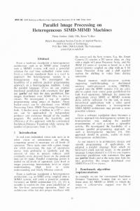
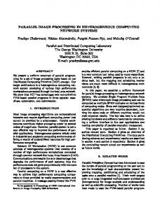
2. COMPUTE UNIFIED DEVICE ARCHITECTURE 2.1 Hardware Device Graphics Processing Units (GPUs) have evolved over the years with a focus on providing the high throughput, low cost devices necessary for the gaming industry. To satisfy such demands, GPU manufacturers (NVIDIA, AMD) talk exclusively with graphics libraries (Direct3D, OpenGL) to ensure maximum hardware acceleration. With the frequent change present in the gaming industry, GPU manufacturers are in rapid release of new models. With each model comes great change within the specific model’s Instruction Set Architecture (ISA). 2.2 GPGPU / CUDA Since the ISAs can change multiple times every year, GPUs have been seemingly impossible to be targeted for any general purpose. NVIDIA’s approach to resolve this problem is the introduction of the Compute Unified Device Architecture (CUDA). CUDA provides the necessary unified programming model for General Purpose GPU (GPGPU) programming. This unified programming model guarantees that any GPU will be able to understand, and execute, any instructions encoded for the CUDA model; regardless of the device’s own ISA. 2.3 GPGPU Considerations The most important aspect of the GPU is the many mechanisms available to turn serial execution into parallel execution. As a prime example, the warp scheduler is in charge of running batches of threads in unison with one another to ensure maximum throughput[4]. The approach to ensuring such optimal throughput include the use of a memory access combination system. Memory access combination refers to the concept of combining memory access among multiple threads; the warp scheduler does so whenever threads access nearby or redundant sections of memory concurrently. If each of the warp’s threads asks for the same location in memory, the warp scheduler performs a single memory read and dispatches that single value to each of the threads. If a grouping of threads access nearby memory locations, the warp scheduler will request a single large section of memory as opposed to requesting multiple small sections of memory for each individual thread[5]. An important note of this system is the reliance on the developer to ensure that these threads work in unison with one another. While the GPU does thrive on parallel execution, serial features are present on the GPU which sometimes perform better than a parallelized approach. A parallelized approach to an inherently serial algorithm often involves combining multiple threads together through the divide-by-half approach (see Fig. 1) [6]. The divide-by-half approach involves combining two threads' results into one result at each iteration; after log2(n) iterations, n number of results have been combined into one result. This parallelized approach provides substantial performance improvements when every thread has its own contribution for the final result.

Figure 1: Parallel Reduction of the serial algorithms through the divide-by-half approach.


2

If an algorithm only needs the combination of a small fraction of the total threads, a parallel reduction approach performs many orders of magnitude slower than an atomic alternative. The atomic alternative utilizes atomic functions that ensure that no two threads will perform the particular function at the same time; eliminating race conditions. Atomic operations require that all threads wait to perform an atomic operation so long as one is being performed. While atomic operations are inherently serial, this is not a concern when the system only requires a small number of atomic operations.

3. THE ATR SYSTEM

3.1 Multi-Stage ATR Architecture

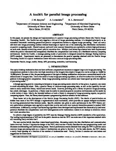
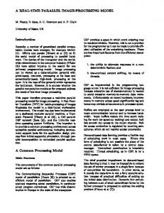
Figure 2: A multi-stage ATR Architecture. JPL has developed a multi-stage ATR system to achieve a balance between speed and accuracy [2]. During preprocessing, a filter is generated using sample images and known ground truths. The filter is also adjusted to the size of the desired target. During the correlation process, the generated composite filter is used to perform a cursory search to quickly find Regions of Interest (ROIs) from the input data. These ROIs are further reduced during the feature extraction process where principle component analysis (PCA) reduces the number of data points that will be used during classification. In the classification process, a Neural Network generates vector outputs which represent whether or not these ROIs contain the desired target.

3.2 Need for Real-Time ATR The ATR system can be considered a valuable tool in the open seas. Peripheral vision is a necessity during navigation, rescue missions, and defense. By applying ATR peripherally to a marine environment, reaction time to emergencies and other sensitive situations should be greatly increased. Seamen who control robotic systems can become overloaded with data, often sifting through hours of streaming video searching for a single ship [7]. Through utilization of an optimized real-time ATR system, these seamen can shift their focus on other matters.

4. COMPOSITE FILTERING

4.1 General Description A composite filter is utilized in this ATR system for cross-correlation between the input image and target. In the test data set, boats were not prone to many of the common filtering problems associated with real world objects. Such problems that were reasonably ignored were scale, rotation and perspective; the test data set showed little reason to accommodate for such disturbances. For such reasons, a composite filtering approach is chosen.


3

4.2 Design Considerations For computation of Fast Fourier Transforms (FFTs) on the GPU, the CUDA model provides the cuFFT library. The cuFFT library performs up to 10x faster than the Math Kernel Library (MKL) provided by Intel for optimized CPU computations [8]. The system must handle scaling the Inverse FFT itself as cuFFT does not innately scale the results. For such scaling, the standard cuBLAS library is utilized.

4.3 Over 24X Performance Boost Performing the composite filter on an image includes the following: Forward FFT, Piecewise Multiplication and Inverse FFT. Considering piecewise multiplication follows the O(n) complexity class, it is clear that the FFTs, being in the O(nlog(n)) complexity class, are the primary consideration in the required computation time. From the dependence on the FFTs, the system is expected to obtain at least the 10x performance boost proposed by the cuFFT library. For the CPU, the FFTs are provided by Numpy’s FFTW-based Discrete Fourier Transform library. For the GPU, the FFTs are provided by the FFTW-based cuFFT library. The average computation time for composite filter cross-correlation requires ~79.7ms on the CPU and ~3.3ms on the GPU. With such speeds, the GPU version performs 24x faster than the CPU version.

5. PEAK FINDING / ROI EXTRACTION

5.1 General Description Cross-correlations produce matrices with varying peaks representing how similar the filter is to the image at that pixel position. It is possible for a system to look for peaks that pass a chosen value; naming a trigger for any peak with a value greater than or equal to the chosen value. The deficit of such a system is the ignorance of the area around the peak; many false triggers would certainly occur while some positive results may never trigger. The chosen ATR system utilizes a peak-to-sidelobe-ratio (PSR) approach to peak finding. As cross-correlations slide across the image, regions with a target should have high peak values at similar locations due to the sliding window. For ROIs, the system should detect very high peak values and clusters of fairly high values bunched together. Such detection is the purpose of the PSR, this ratio is large when the pixel exhibits one (or both) of these features. For the proposed system, a cross-correlative approach obtains such ratios.

5.2 Design Considerations Peak finding is a naturally serial algorithm due to the flexible number of ROIs which may be found. While there are potential approaches to parallelize such an algorithm, the practicality of such parallelization depends on how the system is expected to function. The two major concerns brought on by serial algorithms being executed on the GPU are atomic waits and warp waits. Atomic waits are times where threads on the system must wait for an atomic operation. The atomic waits are a major concern if the system does find many ROIs per image. Warp waits are times where threads must wait for other threads on the warp that are currently active. The warp waits are a major concern if the triggered regions occur individually; if a trigger occurs by itself then approximately 94% of the half-warp is wasted as all other threads are forced to wait. With a peak finder implemented using cross-correlation, a system can take advantage of two important properties of the cross-correlation results. One such feature is the minimalistic nature of results; it is reasonable to expect that the number of pixels that yield high similarities to the filter will be a small fraction of the total pixels. The other


4

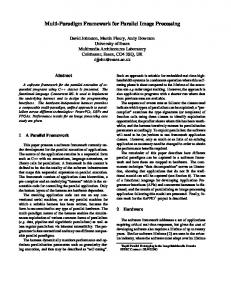
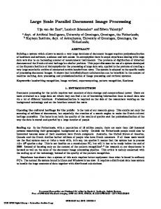
important feature is the locality of triggered regions, which refers to the pattern of cross-correlations to trigger pixels nearby each other. Figure 3 illustrates the correlation peaks found in an image of 1417x256 pixels. Notice such properties in Fig. 3 where the black colors represent triggered peak locations and white colors represent nontriggered pixels; triggered regions being bordered by circles (ROIs) for observability.

Figure 3: Example of the correlation peaks detected by the filtering on an input image.

Figure 3 is an example test image with the correlation peaks triggering a branch in GPU computation. Notice that the majority of pixels are white indicating that the system can safely assume the majority of pixels will skip the branch condition. Even further, the few trigger pixels that will branch will do so in unison with nearby threads as trigger pixels occur in nearby locations. This is observable in Fig. 3 as there is not a heavy dispersion of trigger pixels; trigger pixels occur in clustered regions indicated with bordering circles. With this flow in mind, it is reasonable to use branch conditions for such triggers for GPU computation. As GPUs are Single Instruction Multiple Data (SIMD) devices designed for multiple nearby threads (in a warp) to act in unison, branch conditions can often force non-active threads to wait for active threads. If one of the threads in a half-warp must perform an instruction, all of the instructions in that half-warp must wait for the instruction regardless of their own branching scheme. It is reasonable to branch these conditions inside of a single kernel because the system can assume that the majority of threads will not trigger the branch; most will check and skip the section in unison with each other. The few pixels that will trigger the branch condition should also do so in unison due to the locality of triggered regions; it is inconsiderably rare that a minority of pixels will make the majority of pixels wait. Once peak finder has obtained a list of all center pixels of the ROIs, the system must now extract each ROI’s local bounding area. This function has three major memory considerations: center pixel read, image data read, and ROI data write. For optimization of the center pixel read, nearby threads should access the same center pixel so that the warp scheduler can broadcast this one pixel to all threads in the half-warp. The optimization capabilities of the image data read is limited due to the structure of the image data; which is that of a 2D matrix stored linearly with a width/height separate from the ROI width/height. For optimization, the system must ensure that nearby threads read from nearby indices; the approach to such optimization is reliant on the order of the matrices. For row-major order matrices, the system should ensure that image data is read on a percolumn basis where nearby threads read from the same (or nearby) column. As a consequence of the difference between the ROI height and image height, it is impossible for every thread to read from similar indices; skipping to the next column in the ROI will require a large index jump in the image data.


5

5.3 Over 500X Performance Gain Peak finding requires two FFT based cross-correlations while ROI extraction requires memory reads and writes. As a consequence of relying on custom kernels for ROI extraction, there is no base line for expected performance increase. It is reasonable to assume that performance will be increased due to the cuFFT’s performance increase along with the high memory bandwidths available on GPU devices. The average computation time for Peak finding along with ROI extraction is ~3,247ms on the CPU and ~5.6ms on the GPU. With such speeds, the GPU version performs 580x faster than the CPU version. A majority of the speed increase is accounted for by the high memory bandwidth available on the GPU device. Some of this performance increase is certainly attributed to the unfair comparison of interpreted Python code to compiled C++ code; a reasonable assumption being one order of magnitude.

6. PCA / NEURAL NETWORK

6.1 General Description Principle Component Analysis (PCA) is a procedure of determining components with the highest variance. The use of such components is the reduction of data down to the most important pieces[9]. Such a reduction allows the Neural Network to disregard needless components of the original data. A Neural Network (NN) is chosen for its ability to be trained for classification of complex classes of targets based on existing data. Such training results in matrices, representing weights and biases, which can be used to determine whether or not any new input is a target[10]. In order to use such matrices, a system must perform matrix multiplication and piece-wise addition.

6.2 Design Considerations The results of the PCA matrix multiplication come as a column-major order matrix with a column for every numerical feature and a row for every detected ROI. The activation function consists of matrix multiplication, piecewise addition and hyperbolic tangent. Such an activation function, for the system utilized, is performed twice for every row (every ROI) because of the two layers in the NN. Such activation results can be used to conclude the likelihood of each ROI being a target. A naïve implementation of this system would loop through every column of the PCA matrix, perform the necessary steps and store the result into a temporary matrix. There are multiple deficits in optimization of such a naïve system particularly because of the size of these matrices. Each ROI result from the PCA is a vector of size equal to the numerical feature count. The NN biases and weights are of sizes no greater than the square of the numerical feature count. With such small matrices, the GPU would spend a majority of its time setting up for these kernels to run. An optimized implementation of this system uses batching methods available in cuBLAS in an effort to ensure that each kernel is capable of reaching the ten thousand (or greater) maximum concurrent thread count of GPU devices. The one unfortunate byproduct of batching methods for the GPU device is the necessity of an intricate memory system required by cuBLAS. For batching matrix multiplication, cuBLAS demands an array in device memory containing all of the pointers associated with every individual matrix to be multiplied. This could mean that, for every image, the system must allocate memory on the CPU (host) and GPU (device), fill the host array with matrix pointers and copy such host arrays to the device for cuBLAS. The solution to such an unproductive step is to allocate enough memory to store up to some maximum number of ROIs. For processing an image, the system will use any memory that it needs and ignore any memory that it does


6

not. The practicality of this maximum number, and its value, comes from the ROI height/width and image height/width. It is reasonable to assume that the system, because of the peak finder, will not have any conflicting ROIs where one ROI is inside another. If no ROIs are in conflict with one another, the maximum number of ROIs for any image is equal to the ratio of image size and ROI size. An important note being that this maximum ROI count multiplied by ROI size is equal to the original image size; the system must only reserve memory equal to the input image size to hold any practical number of ROIs.

6.3 Over 17X Performance Gain Performing the PCA and NN activation requires numerous small matrix multiplications. For the CPU, these matrix multiplications are performed by the Numpy and PyBrain libraries available for Python. For the GPU, these matrix multiplications are performed by the cuBLAS library provided by CUDA. The average PCA/Activation consumes computation time of ~6.9ms on the CPU and ~0.6ms on the GPU using the naïve method. While a roughly 11.5x speed boost is certainly appreciated, this system is naïve and can be enhanced. When implemented with the optimized approach, the computation time is ~0.4ms; resulting in a ~17x performance improvement.

7. MULTIPLE GPU (MULTIGPU)

7.1 General Description Typical gaming computers, in present day, are equipped with multiple PCI-Express slots to allow the use of multiple high-speed peripherals. When further speed improvements are required, a system would wisely use these unoccupied slots to supply the system with an additional processor. In terms of cost efficiency, purchasing additional GPUs often yields more processing power than purchasing a single expensive GPU. Another noteworthy improvement provided by a MultiGPU system is the flexibility for further performance with the addition of extra GPUs. For typical gaming PCs, the maximum number of GPUs supported by the motherboard ranges between two and four. Host multithreading is required for the ATR system to utilize multiple GPUs concurrently. For every GPU, there must be a single host thread bound to it and a single host thread can only bind to one GPU at a time. NVIDIA’s CUDA model provides a function (named “cudaGetDeviceCount”) capable of discovering all CUDA capable devices on the machine; a necessity for a program to be flexible with the number of GPUs present on the system. To allow for synchronization of the system’s host threads, common multithreading primitives are utilized. 7.2 Design Considerations The multithreading aspect of the system will primarily be handled by a specialized (and relatively simple) job queue. This job queue has three primary considerations: Thread Setup, Job Insertion, Job Completion. Do note the level of indirection wherein the job queue is handled entirely by host CPU threads while execution of the jobs occurs independent of the job queue. The purpose for this indirection is the flexibility of a MultiGPU system which can be applied to any existing single GPU system; where the single GPU solution performs the task of job processing. While it is possible to separate each of the various stages (PCA, Correlation, etc.) to have a job per stage (JPS), there are many deficits of such a system. The most potent deficit of a JPS system is the memory transfer between GPU devices; necessary for using the output of one stage as the input of the next stage. To transfer values from one GPU to another directly (peer-to-peer), the GPUs must be Tesla models. Tesla models cost around five times as much as typical gaming GPUs. Even with peer-to-peer capabilities available, the JPS system has the deficit of


7

relying on the slow PCI-E bus for memory transfer. Without Tesla devices, the JPS system doubles the inefficiency with the need to initiate a GPU to CPU and CPU to GPU transfer. This memory transfer inefficiency is the JPS system’s downfall; copying memory between the GPUs and host should be reduced whenever possible. The alternative that this ATR system proposes is the single job system. In a single job system, the system must ensure that there will still be plenty of jobs for the system to dispatch to available GPUs. In the ATR system, a single job refers to the processing of a single frame of which is assumed will be plentiful. With such practicalities assumed, the single job system’s one deficit is almost nonexistent. Thread Setup on the system must first allocate global memory which every thread has access to; this memory is for any of the necessary constant data to process incoming jobs. For the ATR system, this global memory primarily consists of a PCA matrix, pre-computed filters and NN weights and biases. The system must then request for the OS to create a thread for every detected GPU on the system; each thread then running a setup function to copy the global memory from host memory to device memory. Job Insertion provides the system with necessary input, output and job types. For the ATR system, job type is excluded due to the system being a single job system. For insertion, the system must ensure that no two threads attempt to add an element concurrently; disabling race conditions. This locking is accomplished with the use of a mutex; a common locking mechanism which can be used to ensure only one instance of an action occurs at a time. This serialization is not a concern for the system’s overall computation time as this step requires many orders of magnitude less time than processing; in the example ATR system, this order of magnitude is around four. Job Completion refers to the extraction and processing of a job from the queue. As with Job Insertion, the system must ensure that the queue is not already being modified by another thread; again, a mutex enforces this rule. Once a job has been extracted from the queue, the mutex is unlocked to allow any other threads to modify the queue. As each job contains a section of memory independent of any other thread (for both input/output), the system can process this job without any fears of race conditions. 7.3 Results of Multiple GPU System With any management scheme comes overhead due to the extra task of ensuring thread cooperation. In the ATR system, this overhead should be relatively small because a job consists of multiple computationally expensive tasks. Processing a frame consumes 9.5ms and thread management consumes 0.2ms per job; equating to a total overhead of 2% for thread management. The primary goal of any MultiGPU approach is to obtain a speed up as additional GPUs are utilized. As a theoretical maximum, the MultiGPU system can process as many frames as the system has GPUs in the same time as it takes a single GPU to process a single frame. For a dual GPU system, 2 GPUs must process two frames in the same time as it takes a single GPU to process a single frame. The MultiGPU system presented in this paper processes a single frame in 9.7ms with a single GPU and two frames in 9.8ms with dual GPUs. As a comparison of processing rates, a single GPU processes approximately 103 frames per second while two GPUs can collectively process approximately 204 frames per second. From such results, additional GPUs provide speedup within 1% of the theoretical maximum.

8. EXPERIMENTAL RESULTS

8.1 System Performance The final system has been optimized to run ~357x faster by retargeting the system to perform the necessary computations on a single GPU rather than the CPU. With the CPU approach, a third of a frame is processed per second. When the same ATR system is developed with the single GPU approach, the system is able to process approximately 105 frames per second. With the MultiGPU approach and two active GPUs, the system is capable


8

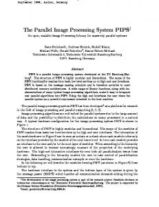
of processing approximately 204 frames per second. JPL has similar algorithms produced from an optimized CPU approach that are able to process five frames per second. See following page for a visualization of such results.

Frames Processed (Per Second)

ATR System Performance 204

210 180 150

105

120 90 60 30

0.3

5

CPU

CPU (Optimized)

0 Single GPU

Dual GPU

Figure 4: ATR System Performance Comparison: Dual GPU system can reach 204 fps, outperforming a regular CPU system > 600X in processing speed for ATR operations.

Results were generated utilizing a fairly typical gaming pc running Windows 8.1 equipped with an Intel i7-3770 CPU ($325), and two NVIDIA GTX 770 GPUs ($370 each). Prices accurate as of February 2013. A considerable concern for an ATR system is the ability to process large fields of view with high frame rates. The test dataset is sourced from a four-camera system where each camera provides a 1417 x 256 sized frame at 20fps. With each frame representing a 90° field of view, these cameras grant a complete 360° field of vision with a combined 80fps. Therefore, to achieve real-time functionality, the ATR system would must process at least 80 frames every second. Using the GPU approach outlined in this paper, a typical gaming pc could process all of this incoming data; with time to spare. This approach is also scalable to larger projects with the flexibility of utilizing additional GPUs to accommodate faster frame rates or additional filtration.

8.2 ATR Examples The following Fig. 5 is an example of the typical output of the system. The inner white box indicates the region for the expected target. The outer dashed white box indicates the zoomed region displayed in Fig. 6.


9

Figure 5: Test Image with Target Detection

Figure 6: Test Image with Target Detection (Zoom)

Accuracy

8.3 ATR System Accuracy

0.8 0.7 0.6 0.5 0.4 0.3 0.2 0.1 0 0

0.02

0.04

0.06

0.08 0.1 0.12 0.14 False Targets Per Image

0.16

0.18

0.2

Figure 7: FROC Curve of Test Images The preceding Free-Response Operator Characteristic (FROC) curve represents the accuracy of the true target detection vs. the number of false alarms per image of the system. As the threshold is decreased for a target value, the system identifies additional true positives while also identifying additional false positives. Notice that changing the threshold value no longer improves accuracy above 70% and significantly increases the number of false targets per image. The primary contributors to the 70% accuracy cap being the limited resolution and boat’s rotations; notice that the level of detail for a boat is very low in Fig. 6. From the FROC curve, the system is able to correctly identify around 70% of the targets while only misidentifying approximately 1 target for every 10 images. While 70% may not seem ideal, keep in mind that this statistic refers to ground truths for every single frame of test data. In a real world system, the large number of frames per second will allow accurate detection of targets within fractions of a second. If the target is on the screen for 3 frames (150ms), the system will correctly identify the target in at least one frame with a 97.3% accuracy. From the test


10

data, boats were visible for at least 6 frames that ensures a single frame detection accuracy of 99.92%; most boats were visible for much longer than 6 frames allowing for even higher accuracy of detection.

9. CONCLUSIONS

This paper provides the design considerations necessary for development of a parallel ATR system platform using the GPU processor. The throughput of such a system is more than capable of providing the necessary computation for robust real-world applications. The application outlined in this paper is a four-camera system providing a 360° field of view around a surface vehicle. For such an application, as well as more robust applications, a typical gaming pc is the only computational necessity. The system is scalable for further complexity with the flexibility of harnessing the power of additional GPUs.

10. ACKNOWLEDGEMENTS The research described in this paper was conducted at the Jet Propulsion Laboratory, California Institute of Technology under a contract with the National Aeronautics and Space Administration. This project was also sponsored by the MSP program through NASA, JPL, and Caltech. Special thanks goes to Jack Fitzsimons, Colin Costello, George Reyes and Rachelle Yongvanich for their continuing guidance, advice, and support.

REFERENCES [1]

Tsung, H-L., Lu, T., Braun, H., Edens, W., Zhang, Y., Chao, T-H., Assad, C., Huntsberger, T., "Optimization of a multi-stage ATR system for small target identification," Proc. of SPIE, 7969 (2010).

[2]

T. Lu, C. Hughlett, H. Zhou, T-H. Chao, and J. Hanan, “Neural network post-processing of grayscale optical correlator,” SPIE Conference 5908 (2005).

[3]

Bathen, L., Bagherzadeh., "A Fast and Innovative Approach Towards an Automatic Target Recognition System Implementation on a Reconfigurable Architecture," http://www.ics.uci.edu/~lbathen/MorphoSys_ATR.pdf (2005).

[4]

Nvidia Corporation, PTX ISA 3.2. “3.1. A Set of SIMT Multiprocessors with On-chip Shared Memory” http://docs.nvidia.com/cuda/parallel-thread-execution/index.html (2013).

[5]

Jog, A., Kayiran, O., Nachiappan, N., Mishra, A., Kandemir, M., Mutlu, O., Iyer, R., Das, C., “OWL: Cooperative Thread Array Aware Scheduling” (2013). Page 3. http://www.cse.psu.edu/~axj936/docs/OWL-ASPLOS-2013.pdf (2013).

[6]

CUDA Parallel Reduction Figure. Tech 621 Schedule; Purdue University, http://tech621.tech.purdue.edu/schedule.htm (2013).

[7]

Jean, G., "Pirates, Beware: Navy's Smart Robocopters Will Spy You in the Crowd," http://www.onr.navy.mil/Media-Center/Press-Releases/2012/Unmanned-Sensor-Automatic-TargetRecognition.aspx (2012).

[8]

Nvidia Corporation, Nvidia Developer Zone: cufft, http://www.developer.nvidia.com/cufft (2006).

[9]

Shlens, J., "A tutorial on principal component analysis," http://www.snl.salk.edu/~shlens/pca.pdf (2009).


11

[10]

Ye, D., Edens, W., Lu, T., Chao, T-H., "Neural network target identification system for false alarm reduction," Proc. of SPIE, 7340 (2009).


12