Graph Construction for Learning with Unbalanced Data

Graph Construction for Learning with Unbalanced Data

arXiv:1112.2319v1 [stat.ML] 11 Dec 2011

Jing Qian Boston University Boston, MA 02215

Venkatesh Saligrama Boston University Boston, MA 02215

Abstract Unbalanced data arises in many learning tasks such as clustering of multi-class data, hierarchical divisive clustering and semi-supervised learning. Graph-based approaches are popular tools for these problems. Graph construction is an important aspect of graph-based learning. We show that graph-based algorithms can fail for unbalanced data for many popular graphs such as k-NN, ǫ-neighborhood and full-RBF graphs. We propose a novel graph construction technique that encodes global statistical information into node degrees through a ranking scheme. The rank of a data sample is an estimate of its p-value and is proportional to the total number of data samples with smaller density. This ranking scheme serves as a surrogate for density; can be reliably estimated; and indicates whether a data sample is close to valleys/modes. This rank-modulated degree(RMD) scheme is able to significantly sparsify the graph near valleys and provides an adaptive way to cope with unbalanced data. We then theoretically justify our method through limit cut analysis. Unsupervised and semi-supervised experiments on synthetic and real data sets demonstrate the superiority of our method.

1

Introduction and Motivation

Graph-based approaches are popular tools for unsupervised clustering and semi-supervised (transductive) learning(SSL) tasks. In these approaches, a graph representing the data set is constructed. Then a graph-

Manqi Zhao Google Inc. Mountain View, CA

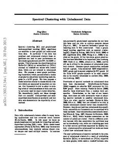
based learning algorithm such as spectral clustering(SC) ([1], [2]) or SSL algorithms ([3], [4], [5]) is applied on the graph. These algorithms solve the graphcut minimization problem on the graph. Of the two steps, graph construction is believed to be critical to the performance and has been studied extensively([6], [7], [8], [9], [10]). In this paper we will focus on graphbased learning for unbalanced data. The issue of unbalanced data has independent merit and arises routinely in many applications including multi-mode clustering, divisive hierarchical clustering and SSL. Note that while model-based approaches([11]) incorporate unbalancedness, they typically work well for relatively simple cluster shapes. In contrast non-parametric graph-based approaches are able to capture complex shapes([2]). Common graph construction methods include ǫ-graph, fully-connected RBF-weighted(full-RBF) graph and knearest neighbor(k-NN) graph. ǫ-graph links two nodes u and v if d(u, v) ≤ ǫ. ǫ-graph is vulnerable to outliers due to the fixed threshold ǫ. Full-RBF graph links every pair with RBF weights w(u, v) = exp(−d(u, v)2 /2σ 2 ), which is in fact a soft threshold compared to ǫ-graph(σ serves the similar role as ǫ). Therefore it also suffers from outliers. k-NN graph links u and v if v is among the k closest neighbors of u or vice versa. It is robust to outlier and is the most widely used method.([7], [6]). In [9] the authors propose b-matching graph. This method is supposed to eliminate some of the spurious edges that appear in k-NN graph and lead to improved performance([10]). Nevertheless, it remains unclear what exactly are spurious edges from statistical viewpoint? How does it impact graph-based algorithms? While it is difficult to provide a general answer, the underlying issues can be clarified by considering unbalanced and proximal clusters as we observe in many examples. Example: Consider a data set drawn i.i.d from a proximal P2 and unbalanced 2D gaussian mixture density, i=1 αi N (µi , Σi ), where α1 =0.85, α2 =0.15, µ1 =[4.5;0], µ2 =[-0.5;0], Σ1 = diag(2, 1), Σ2 = I. Fig.1 shows different graphs and clustering results. SC fails

Graph Construction for Learning with Unbalanced Data

8

4 Cut on k−NN RatioCut on k−NN RatioCut on ε−graph RatioCut on full−RBF RatioCut on RMD

0.08 6 0.06

0 −2

5 Graph Cut

x =1 1

0.04

2 x2

7

0.02

−4 −6

−4

−2

0

2

4

6

8

10

−4

−2

0

2 x1

4

6

8

10

4 4 3 2

0

x2

2 2 0 −2

−2

x2

4

2

0

6

8

0 −4

x1

−2

0

2

4

6

8

−4 −6

10

(b) graph cuts of hyperplanes along x1

(c) ǫ-graph and full-RBF graph 4

2

2

2

0

−4 −6

x2

4

x2

4

−2

0 −2

−4

−2

0

2

4

6

8

−4 −6

10

0 −2

−4

−2

0

2

4

6

8

−4 −6

10

4

4

2

2

2

0 −2 −4 −6

x2

4

x2

x2

0 −2

x1

(a) pdf

x2

1

0 −2

−4

−2

0

2 x1

4

6

8

10

(d) k-NN graph

−4 −6

−4

−2

0

2

4

6

8

10

−4

−2

0

2 x1

4

6

8

10

0 −2

−4

−2

0

2 x1

4

6

(c) b-matching graph

8

10

−4 −6

(d) our method(RMD graph)

Figure 1: Graphs and SC results of unbalanced 2-Gaussian density. Graph cut curves in (b) are properly rescaled. Full-RBF graph is not shown. Binary weights are adopted on ǫ-graph, k-NN, b-matching and RMD graph. The clustering results on full-RBF and ǫ-graph are exactly same. The valley cut is approximately x1 ≈ 1. SC fails on ǫ-graph and full-RBF graph due to outliers. SC on k-NN or b-matching graph cuts at the balanced position due to impact of the balancing term. Our method significantly prunes spurious edges near the valley, enabling SC to cut at the valley, while maintaining robustness to outliers. on ǫ-graph and full-RBF graph due to outliers; SC on k-NN(b-matching) graph cuts at the wrong position.

when dealing with intrinsically unbalanced and proximal data sets.

Discussion: To explain this phenomenon, we inspect SC from the viewpoint of graph-cut. G = (V, E) is the graph constructed from data set with n samples. ¯ as a 2-partition of V separated by a Denote (C, C) given hyperplane S. The simple cut is defined as: X ¯ = w(u, v) (1) Cut(C, C)

As a whole, the existing graph construction methods on which the graph-based learning is based have the following weaknesses:

¯ w∈C,v∈C,(u,v)∈E

where w(u, v) is the weight of edge (u, v) ∈ E. To avoid the problem of singleton clusters, SC attempts to minimize the RatioCut or Normalized Cut(NCut):   1 1 ¯ ¯ + ¯ (2) RatioCut(C, C) = Cut(C, C) |C| |C|   1 1 ¯ ¯ + NCut(C, C) = Cut(C, C) (3) ¯ vol(C) vol(C)

where |C| denotes the number of nodes in C, vol(C) = P u∈C,v∈V w(u, v). Note that RatioCut(NCut) adds to the Cut(we will keep using Cut throughout our paper to denote the simple cut) with a balancing term, which in turn induces partitions to be balanced. While this approach works well in many cases, minimizing RatioCut(NCut) on k-NN graph has severe drawbacks

(1) Vulnerability to Outliers: Fig.1(b) shows that both the RatioCut curves on ǫ-graph(cyan) and fullRBF graph(green) and the Cut curve(black) are all small at the boundaries. This means in many cases seeking global minimum on these curves will incur single point clusters. It is relatively easy to see that the Cut value is small at boundaries since there is no balancing term. However, it is surprising that even for this simple example, ǫ-graph and full-RBF graph are vulnerable to outliers(Fig.1(c)), even with the balancing term. This is because the Cut value is zero for ǫ-graph and exponentially small for full-RBF. k-NN graph does not suffer from this problem and is robust to outliers. (2) Balanced Clusters: The k-NN graph while robust results in poor cuts when the clusters are unbalanced. Note that the valley of the k-NN Cut curve(black) corresponds to the density valley(x1 = 1 in Fig.1(b)) is the optimal cut in this situation. How-

Jing Qian, Venkatesh Saligrama, Manqi Zhao

ever, the red curve in Fig.1(b) shows that the minimum RatioCut on k-NN graph(similar on b-matching graph) is attained at a balanced position(x1 = 3.5). Example Continued: To understand this drawback of k-NN graph, consider a numerical analysis on this example. Assume the sample size n is sufficiently large and k properly chosen such that k-NN linkages approximate the neighborhoods of each node. Then there are roughly knS edges near the separating hyperplane S, where nS is the number of S. Empiri points along  1 1 cally RatioCut(S) ≈ knS |C| + |C| on unweighted ¯

k-NN graph. Let S1 be the valley cut(|C|/|V | = 0.15), which corresponds to x1 ≈ 1; S2 be the balanced cut(|C|/|V | = 0.5), x1 ≈ 3.5. Let n1 and n2 be the number of points within a k-neighborhood of S1 and S2 respectively. It follows that RatioCut1 ≈ 7.84kn1 /n and RatioCut2 ≈ 4kn2 /n. SC will erroneously prefer S2 rather than the valley cut S1 if n2 < 1.96n1 . Unfortunately, this happens very often in this example since the data set is unbalanced and proximal. We ascribe this observation to two reasons: (a) RatioCut(NCut) Objective: RatioCut(NCut) does not necessarily achieve minimum at density valleys. The minimum is attained as a tradeoff between the Cut and the sizes of each cluster(balancing term). While this makes sense when the desired partitions are approximately balanced, it performs poorly when the desired partitions are unbalanced, as shown in Fig.1(d),(e).

(b) Graph Construction: k-NN(b-matching) graph does not fully account for underlying density. Primarily, density is only incorporated in the number of data points along the cut. The degree of each node is essentially a constant and does not differentiate between high/low density regions. This can be too weak for proximal data. Indeed, [12] also argues that k-NN graph only encodes local information and the clustering task is achieved by pulling all the local information together. In addition, we also observe this phenomena from the limit cut on k-NN graph [8]:   Z 1 1 (4) + constant · f 1−1/d (s)ds µ(C) µ(V \C) S R where µ(C) = C f (x)dx, f the underlying density, d the dimension. The limit of the simple Cut R f (s)ds(even without the weakening power of d) only S counts the number of points along S. There is no information about whether S is near valleys/modes. While other graphs limits of R R do incorporate more density(the Cut are S f 2 (s)ds for ǫ-graph [8] and S f (s)ds for full-RBF graph [13]), they are vulnerable to outliers and their performance is unsatisfactory for both balanced and unbalanced data as in [10] and our simula-

tions. Our Approach: The question now is how to find the valley cut while maintaining robustness to outlier? At a high-level we would like to follow the density curve while avoiding clusters that correspond to outliers. One option can be to improve the objective,  1 1 2 on k-NN for example, minimize cut (S) |C| + |C| ¯ graph. However, it is unclear how to solve this problem. We adopt another approach, which is to construct a graph that incorporates the underlying density and is robust to outliers. Specifically, we attempt to adaptively sparsify the graph by modulating node degrees through a ranking scheme. The rank of a data sample is an estimate of its p-value and is proportional to the total number of samples with smaller density. This rank indicates whether a node is close to density valleys/modes, and can be reliably estimated. Our rankmodulated degree(RMD) graph is able to significantly reduce(increase) the Cut values near valleys(modes), leading to emphasizing the Cut in RatioCut optimization, while maintaining robustness to outliers. Moreover, our scheme provides graph-based algorithms with adaptability to unbalanced data. Note that success in clustering unbalanced data has implications for divisive hierarchical clustering with multiple clusters. In this scheme at each step a binary partition is attained by SC with possibly two unbalanced parts. The remainder of the paper is organized as follows. We describe our RMD scheme for learning with unbalanced data in Sec.2, with more details in Sec.2.1∼2.4. The limit expression of RatioCut(NCut) for RMD graph is investigated in Sec.3. Experiments on synthetic and real datasets are reported in Sec.4.

2

RMD Graph: Main Idea

We propose to sparsify the graph by modulating the degrees based on ranking of data samples. The ranking is global and we call the resulting graph the Rank-Modulated Degree(RMD) graph. Our graph is able to find the valley cut while being robust to outliers. Moreover, our method is adaptable to data sets with different levels of unbalancedness. The process of RMD graph based learning involves the following steps: (1) Rank Computation: The rank R(u) of node (data sample) u is calculated: R(u) =

N 1 X I{G(u)≤G(xi )} N i=1

(5)

where I denotes the indicator function, G(u) is some statistic of u. The rank is an ordering of the data samples based on statistic G(·).

Graph Construction for Learning with Unbalanced Data

(2) RMD Graph Construction: Connect each node u to its deg(u) closest neighbors, where the degree is modulated through an affine monotonic function of the rank:

2

x

0 −2

(6)

−4 −4

−2

0

2

4

6

8

10

8

10

4 0.1

0.3 0.1

−2 −4 −4

0.7

0.3

0.1 −2

0

0.3 0.7

0.1

0.3

0.1

0

0.5

2

2

0.5

where k is the average degree, φ is some monotonic function and λ ∈ [0, 1]. (3) Graph-based Learning Algorithms: Spectral clutering or graph-based SSL algorithms, which involves minimizing RatioCut(NCut), are applied on RMD graph. (4) Cross-Validation Scheme: Repeat (2) and (3) using different configurations of degree modulation scheme(Eq.(6)). Among the results, pick the best which has the minimum simple Cut value. 2.1

2

x

deg(u) = k(λ + φ(R(u)))

4

2

4

6

x

1

pdf vs rank Figure 2: pdf and ranks of the unbalanced 2-Gaussian density of Fig.1. High/low ranks correspond to density modes/valleys.

Rank Computation

We have several options for choosing the statistic G(·) for rank computation. (1) ǫ-Neighborhood: Choose an ǫ-ball around u and set: G(u) = −Nǫ (u), where Nǫ (u) is the number of neighbors in an ǫ radius of u. (2) l-Nearest Neighorhood: Here we choose the l-th nearest-neighbor distance of u: G(u) = D(l) (u). (3) Average l-Neighbor distance: The average of u’s 2l -th to 3l 2 -th nearest-neighbor distances: 1 G(u) = l

l+⌊ 2l ⌋

X

D(i) (u)

(7)

i=l−⌊ l−1 2 ⌋

Empirically we observe the third option leads to better performance and robustness. For the purpose of implementation (see Sec. 4) we use the U-statistic resampling technique for reducing variance([14]). Properties of Rank Function: (1) Valley/Mode Surrogate: The value of R(u) is a direct indicator of whether u lies near density valleys.(see Fig.2). It ranges in [0, 1] with small values indicating globally low density regions and large values indicating globally high-density regions. (2) Smoothness: R(u) ∈ [0, 1] is the integral of pdf asymptotically(see Thm.1 in Sec.3); it’s smooth and uniformly distributed. This makes it appropriate to globally modulate the degrees of nodes without worrying about scale and allows controlling the average degree. (3) Precision: We do not need our estimates to be precise for every point; the resulting cuts will typically depend on low ranks rather than the exact value, of most nearby points.

2.2

Rank-Modulated Degree Graph

Based on the ranks, our degree modulation scheme(Eq.(6)) successfully solves the two issues of traditional graphs, as well as additionally provides the adaptability to data sets with different unbalancedness: (1) Emphasis of Cut term: The monotonicity of deg(u) in R(u) immediately implies that nodes near valleys(with small ranks) will have fewer edges. Fig.1(b) shows that compared to k-NN graph, RMD graph significantly reduces(increases) Cut(thus RatioCut) values near valleys(modes), and RatioCut minimum is attained near valleys. Fig.1(f) demonstrates the remarkable effect of graph sparsification near density valleys on RMD graph. Example Continued: Recall the example of Fig.1. On RMD graph RatioCut1 ≈ 7.84k1 n1 /n and RatioCut2 ≈ 4k2 n2 /n, where k1 and k2 are the average degrees of nodes around the valley cut S1 (x1 = 1) and the balanced cut S2 (x1 = 3.5). Fig.2 shows the average rank near S1 is roughly 0.2 and 0.7 near S2 . Suppose the degree modulation scheme is deg(u) = k(1/3 + 2R2 (u)), then k1 ≈ 0.41k and k2 ≈ 1.31k. Now S2 is erroneously preferred only if n2 < 0.61n1 , which hardly happens! (2) Robustness to Outliers: The minimum degree of nodes in RMD graph is kλ, even for distant outliers. This leads to robustness as is shown in Fig.1(b), where the RatioCut curve on RMD graph(blue) goes up at border regions, guaranteeing the valley minimum is the global minimum of RatioCut. Fig.1(f) also shows SC on RMD graph works well with the outlier. (3) Adaptability to Unbalancedness: The parameters in Eq.(6) can be configured flexibly. With

Jing Qian, Venkatesh Saligrama, Manqi Zhao

our cross-validation scheme, this degree modulation scheme can offer graph-based learning algorithms with adaptability to data sets with different unbalancedness. We’ll discuss this advantage in Sec.2.4. To construct RMD graph, we provide two algorithms. The first is similar to the traditional k-NN: connect u and v if v is among the deg(u) nearest neighbors of u or u is among the deg(v) nearest neighbors of v. We determine the degree for each node based on Eq. 6. The time complexity is O(n2 logn). The second method solves an optimization problem to construct RMD graph: X Pij Dij (8) min Pij ∈{0,1}

s.t.

X j

ij

Pij = deg(xi ), ∀i, j ∈ 1, ..., n

Details about SC can be found in [7]. Gaussian Random Fields(GRF): GRF aims to recover the classification function F = [Fl Fu ]T by optimizing the following cost function on the graph: min tr(F T LF )

F ∈Rn×c

s.t. LFu = 0, Fl = Yl where c is the number of classes, L denotes the unnormalized graph Laplacian, Yl the labeling matrix. Details about GRF can be found in [3]. Graph Transduction via Alternating Minimization(GTAM): Based on the graph and label information, GTAM aims to recover the classification function F = [Fl Fu ]T ∈ Rn×c where Fl (Fu ) corresponds to the labeled (unlabeled) data. Specifically, GTAM solves the following problem: min tr(F T LF + µ(F − V F )T (F − V Y )) F,Y X Yij = 1 s.t.

Pii = 0, Pij = Pji , ∀i, j ∈ 1, ..., n where Dij is the distance between xi and xj , Pij = 1 indicates an edge between xi and xj . Different distance metrics can be applied such as the Euclidean distance or other derived distance measures. To solve this optimization problem, we apply the Loopy Belief Propagation algorithm which is originally designed for the b-matching problem in [15]. They prove that max-product message passing is guaranteed to converge to the true maximum MAP in O(n3 ) time on bipartite graphs; in practice the convergence can be much faster. More details can be found in [15]. 2.3

Graph Based Learning Algorithms

We apply several popular graph-based algorithms on various graphs to validate the superiority of RMD graph for unsupervised clustering and semi-supervised learning tasks. These algorithms all involving minimizing tr(F T LF ) plus some other constraints or penalties, where F is the cluster indicator function or classification(labeling) function, L is the graph Laplacian matrix. Based on spectral graph theory [16], this is equivalent to minimizing RatioCut(NCut) for unnormalized(normalized) L. Spectral Clustering(SC): Let n denotes the sample size, c the number of clusters, Cj the j-th cluster, j = 1, ..., c, and L the unnormalized graph Laplacian matrix computed from the constructed graph. F is the cluster indicator matrix. Unnormalized SC(NCut minimization for normalized L is similar) aims to solve the following optimization problem: min tr(F T LF ) F

s.t. F T F = I, F as defined above.

j

where V is a node regularizer to balance the influence of labels from different classes. Details about GTAM can be found in [5]. 2.4

Adaptability and Cross Validation Scheme

Parameters in Eq.(6) can be specified flexibly. Our overall approach is to keep the average degree at k, while sparsifying the graph differently to cope with unbalanced data. Note that R(u) is uniformly distributed within [0, 1] and φ is any monotonic function. For example, if φ equals identity and λ = 0.5, the node degrees deg(u) = k(0.5+R(u)) and the degree range is [ 21 k, 32 k]; another example is deg(u) = k(1/3 + 2R2(u)) with node degrees in [ 13 k, 73 k]. Generally speaking, RMD graphs with small dynamic ranges of node degrees lead to less flexibility in dealing with unbalanced data but are robust to outliers(k-NN is the extreme case where all nodes have same degrees). RMD graphs with large dynamic range lead to sparser graphs and can adapt to unbalanced data. Nevertheless it is sensitive to outliers and can incur clusters of very small sizes. Based on the analysis in Sec.1 and Fig.1(b), we wish to find minimum cuts with sizable clusters. The most important aspect of our scheme is that it adapts to different levels of unbalancedness. We can then use a cross validation scheme to select appropriate cuts. In our simulation, the cross-validation scheme is simple. Among all the partitions obtained by graphbased algorithms on several different RMD graphs, we

Graph Construction for Learning with Unbalanced Data

first discard those results with clusters of sizes smaller than a certain threshold(outliers influence the results). Among the rest, we pick the partition with the minimum Cut value.

3

Analysis

Assume the data set D = {x1 , ..., xn } is drawn i.i.d. from density f in Rd . f has a compact support C. Let G = (V, E) be the RMD graph. Given a separating hyperplane S, denote C + ,C − as two subsets of C split by S, ηd the volume of unit ball in Rd . We first show that our ranking acts as an indicator of valley/mode. Regularity condition: f (·) is continuous and lowerbounded: f (x) ≥ fmin > 0. It is smooth, i.e. ||∇f (x)|| ≤ λ, where ∇f (x) is the gradient of f (·) at x. Flat regions are disallowed, i.e. ∀x ∈ X, ∀σ > 0, P {y : |f (y) − f (x)| < σ} ≤ M σ, where M is a constant. First we show the asymptotic consistency of the rank R(u). The limit of R(u), p(u), is exactly the complement of the volume of the level set containing u. Note that p(u) is small near valleys. It is also smoother than pdf, and scales in [0, 1]. The proof can be found in the supplementary material. Theorem 1. Assume the density f satisfies the above regularity assumptions. For a proper choice of parameters of G(u), we have, Z f (x)dx (9) R(u) → p(u) := {x:f (x)≤f (u)}

as n → ∞. Next we study graph-cut induced on unweighted RMD graph. We show that the limit cut expression on RMD graph involves a much stronger and adjustable term. This implies the Cut values near modes can be significantly more expensive relative to those near valleys. For technical simplicity, we assume RMD graph ideally connects each point x to its deg(x) closest neighbors. Theorem 2. Assume the smoothness assumptions in [8] hold for the density f , and S is a fixed hyperplane in Rd . For unweighted RMD graph, let the degrees of point x be: deg(x) = kn (λ + φ(Rl (x))), where λ is the constant bias, and denote the limiting expression ρ(x) := (λ + φ(p(x))). Assume kn /n → 0. In √ case d=1, assume kn / n → ∞; in case d ≥2 assume kn / log n → ∞. Then as n → ∞ we have that: r n d NCutn (S) −→ kn Z
1 1 Cd f 1− d (s)ρ(s)1+ d ds µ(C + )−1 + µ(C − )−1 . S

(10)

satisfied almost surely. (Cd = R f (x)dx.) C±

2ηd−1 1+1/d , (d+1)ηd

µ(C ± ) =

Proof. We only present a brief outline of the proof. We want to establish the convergence result of the cut term and the balancing terms respectively, that is: r Z 1 d n 1 1 cutn (S) → Cd f 1− d (s)ρ(s)1+ d ds. (11) nkn kn S 1 1 → . (12) nkn vol(D± ) µ(C ± ) where D+ (D− ) = {x ∈ D : x ∈ C + (C − )} are the discrete version of C + (C − ). Equation 11 is established in two steps. First we can show that  the  converges to its expectaq LHS cut term 1 d n tion E nkn kn cutn (S) by making use of the con-

centration of measure inequality [17]. Second we show that this expectation term actually converges to the RHS of Equation 11. This is the most intricate part and we state it as a separate result in Lemma 3.

+ For equation 12, P recall that the volume term of D + is vol(D ) = u∈D+ ,v∈D 1. It can be shown that as n → ∞, the distance between any connected pair (u, v) goes to zero. Next we note that the number of points in D+ is binomially distributed Binom(n, µ(C + )). Using the Chernoff bound of binomial sum we can show that almost surely Equation 12 holds true.

Lemma 3. Given the assumptions of Theorem 2,   r Z 1 1 1 d n cutn (S) −→ Cd f 1− d (s)ρ(s)1+ d ds. E nkn kn S where Cd =

4

2ηd−1 1+1/d

(d+1)ηd

.

Simulations

We present experiments to show the power of RMD graph. We focus on the unbalanced settings by sampling the data set in an unbalanced way. First, we use U-statistic resampling technique and obtain averaged ranks with reduced variance [14]. U-statistic Resampling For Rank Computation: We input n = 2m data points, nearest-neighbor parameter l, number of resampling times b. We then Randomly split the data set into two equal parts: S1 = {x1 , ..., xm }, S2 = {xm+1 , ..., x2m }. Then points points in S2 are used to calculate the statistics G(xi ) of xi ∈ S1 and vice versa. The ranks of xi ∈ S1 within S1 and ranks of xi ∈ S2 within S2 , based on Eq.5. We then resample and repeat the steps b times and average to obtain averaged ranks for the data points.

Jing Qian, Venkatesh Saligrama, Manqi Zhao

The algorithm turns out to be robust to the nearestneighbor parameter l. √ In our simulations we select l to be of the order of m. We set the parameter of resampling times b = 10 in our experiments. Note that the complexity of rank calculation is O(bn2 logn). Other general parameters are specified below: (1) In the rank R(u), we choose the statistic G(u) as in Eqn.7. The ranks are quite robust to the choice of parameter l; here we fix l = 50. (2) In the step of U-statistic rank calculation, we fix the resampling times b = 10. (3) We adopt three RMD schemes: (a) deg(u) = k(1/2 + R(u)); (b) deg(u) = k(1/3 + 2R2 (u)); (c) deg(u) = k(1/4 + 3R3 (u)). The average degree k(same as in k-NN or b-matching) will be specified later. (4) For graph construction, both methods described in Sec.2.2 are applied to build RMD graphs. We find the performances are almost the same. So for consideration of complexity, we recommend the simple k-NN style algorithm to build RMD graphs. (5) For cross-validation, we find all clusters returned on RMD graphs of step (3) are sizable. Among these we pick the partition with the minimum Cut value. (6) All error rate results are averaged over 20 trials. 4.1

Synthetic Experiments

0.18

0.24 0.22

0.16

0.12

k−NN graph b−matching graph RMD(deg(u)=k(1/2+R(u)))

0.2 k−NN graph b−matching graph RMD(deg(u)=k(1/2+R(u)))

0.18 error rates

error rates

0.14

2

RMD(deg(u)=k(1/3+2R (u))) 0.1

RMD(deg(u)=k(1/3+2R2(u)))

0.16 0.14

0.08

0.12

0.06

0.04 10

0.1

20

30

40 50 60 k−NN parameter

70

80

90

0.08 10

20

30

40 k−NN parameter

50

60

70

(a) SC on various graphs (b) GTAM on various graphs

Figure 4: SC and GTAM on unbalanced pdf of Fig.1. RMD graph outperforms k-NN or b-matching graph.

2D Examples: We revisit the example discussed in Sec.1. We apply SC, GRF and GTAM on this unbalanced density; the results are shown in Fig.4. Sample size N = 500; binary weights are adopted. For GRF and GTAM there are 20 randomly chosen labeled samples guaranteeing at least one from each cluster, and GTAM parameter µ = 0.05. In both experiments RMD graph significantly outperforms k-NN and b-matching graphs. Notice that different RMD graphs have different power to cope with unbalanced data. Multiple Cluster Example: Consider a data set composed of 2 gaussian and 1 banana-shaped proximal clusters. We manually add an outlier point. SC fails on ǫ-graph(similar on full-RBF graph) because the outlier point forms a singleton component. SC cuts at the balanced positions on k-NN(b-matching) graph instead

of the valley on RMD graph. Divisive Hierarchical Clustering: For situations that require a structural view of the data set, we propose a divisive hierarchical way of performing SC. This is possible because our graph sparsification accounts for unbalanced data and so we can use spectral clustering on RMD for divisive clustering. At every step, the algorithm tries to split each existing part into 2 clusters and computes the corresponding graph cut values. The part with the smallest binary cut value is split until the expected number of clusters is reached. Fig.5 shows a synthetic example composed of 4 clusters. SC on k-NN graph fails at the first cut due to unbalancedness. On RMD graph at each step the valley cut is attained for the sub-cluster from the previous step with the smallest RatioCut value. 4.2

Real DataSets

We focus on 2-cluster unbalanced settings and consider several real data sets from UCI repository. We construct k-NN, b-match, full-RBF and RMD graphs all combined with RBF weights, but do not include the ǫgraph because of its overall poor performance. For all the experiments, sample size n = 750, average degree k = 30. The RBF parameter σ is set to be the average k-NN distance. GTAM parameter µ = 0.05([10]). For SSL algorithms 20 randomly labeled samples are chosen with at least one from each class. Varying Unbalancedness: We start with a comparison, for 8vs9 of the 256-dim USPS digit data set. We keep the total sample size as 750, and vary the unbalancedness, i.e. the proportion of numbers of points from two clusters, denoted by n8 , n9 . Fig.6 shows that as the unbalancedness increases, the performance severely degrades on traditional graphs. RMD graph with deg(u) = k(1/3 + 2R2 (u)) has a stronger effect of emphasizing the Cut, and thus adapts to unbalancedness better than RMD graphs with deg(u) = k(1/2 + R(u)). Other UCI Data Sets: We fix 150/600 samples of two classes which amounts to an unbalancedness fraction of 1 : 4 for several other UCI data sets. Results for RMD graph are obtained through the cross-validation scheme(Sec.2.4). Tab.1,2 shows that our method consistently outperforms other graphss, sometimes overwhelmingly when the data set is unbalanced.

Graph Construction for Learning with Unbalanced Data

5

5

5

4

4

4

3

3

3

2

2

2

1

1

1

0

0

0

−1

−1

−1

−2

−2

−2

−3

−3

−3

−4 −6

−4 −6

−4

−2

0

2

4

6

−4

(a) ǫ-graph

−2

0

2

4

−4 −6

6

(b) k-NN graph

−4

−2

0

2

4

6

(c) RMD graph

Figure 3: 2 gaussian and 1 banana-shaped proximal data set. SC fails on ǫ-graph due to the outlier cluster, cuts at the balanced positions on k-NN graph while at the valley on RMD graph. 6

6

6

6

4

4

4

4

2

2

2

2

0

0

0

0

−2

−2

−2

−2

−4

−4

−6

−6

−4

−4 RatioCut =0.0029819 RatioCut =0.0091047 RatioCut =0.11551

−6 RatioCut =0.0021807 RatioCut =0.11551

−8 −6

−4

−2

0

2

4

−8 −6

6

(a) 1st partition(k-NN)

−4

−2

0

2

4

6

(b) 1st partition(RMD)

−8 −6

−4

−2

0

2

4

RatioCut =0.13704 RatioCut =0.069503 RatioCut =0.11551 RatioCut =0.0091047

−6

−8 −6

6

(c) 2nd partition(RMD)

−4

−2

0

2

4

6

(d) 3rd partition(RMD)

Figure 5: Divisive Hierarchical SC is performed on k-NN and RMD graph of 4-cluster data. Binary cuts are performed until the number of clusters reaches 4. Notice every step involves unbalanced data. k-NN graph fails at the first step. On RMD graph valley cuts are attained at each step. 0.6

0.3

0.3 k−NN b−matching full−RBF RMD(deg(u)=k(1/2+R(u)))

0.5

k−NN b−matching full−RBF RMD(deg(u)=k(1/2+R(u)))

0.25

RMD(deg(u)=k(1/3+2R2(u)))

RMD(deg(u)=k(1/3+2R2(u))) 0.4

RMD(deg(u)=k(1/3+2R2(u))) 0.2

0.3

error rates

0.2 error rates

error rates

k−NN b−matching full−RBF RMD(deg(u)=k(1/2+R(u)))

0.25

0.15

0.2

0.15

0.1 0.1

0.1

0.05 0.05

0

1

2

3 4 Unbalanceness (n9/n8)

(a) SC on USPS 8vs9

5

6

1

2

3 4 Unbalanceness (n9/n8)

5

(b) GRF on USPS 8vs9

6

0

1

2

3 4 Unbalanceness (n9/n8)

5

6

(c) GTAM on USPS 8vs9

Figure 6: SC, GRF and GTAM on 8vs9 of USPS digit dataset with various mixture proportions. k-NN or b-matching graphs fail. RMD graph with deg(u) = k(1/3 + 2R2 (u)) can adapt to unbalanced data better than with deg(u) = k(1/2 + R(u)).

References [1] J. Shi and J. Malik, “Normalized cuts and image segmentation,” IEEE Transactions on Pattern Analysis and Machine Intelligence, vol. 22, no. 8, pp. 888–905, 2000. [2] A. Y. Ng, M. I. Jordan, and Y. Weiss, “On spectral clustering: Analysis and an algorithm,” in Advances in Neural Information Processing Systems 14. MIT Press, 2001, pp. 849–856. [3] X. Zhu, Z. Ghahramani, and J. Lafferty, “Semi-

supervised learning using guassian fields and harmonic functions,” in International Conference on Machine Learning, 2003, pp. 912–919. [4] D. Zhou, O. Bousquet, T. Lal, J. Weston, and B. Sch¨ olkopf, “Learning with local and global consistency,” in The Neural Information Processing Systems. MIT Press, 2004, pp. 321–328. [5] J. Wang, T. Jebara, and S. Chang, “Graph transduction via alternating minimization,” in International Conference on Machine Learning, 2008.

Jing Qian, Venkatesh Saligrama, Manqi Zhao

Table 1: SC on various graphs of unbalanced real data sets. Results of RMD are obtained after cross-validation. RMD graph performs significantly better than other methods.

Err Rates(%) Waveform 1vs2 Pendigit 6vs8 Pendigit 9vs8 USPS 8vs6 USPS 8vs9 SatLog 1vs7 SatLog 4vs3 LetterRec 6vs7 LetterRec 4vs10

k-NN 12.83 14.95 12.23 4.67 47.05 7.28 20.20 12.45 28.29

b-match 11.03 15.00 12.33 4.52 46.47 7.44 17.79 10.95 29.85

full-RBF 10.35 10.61 14.53 22.83 19.95 9.12 13.69 25.01 25.19

RMD 6.45 4.57 3.53 1.13 3.40 4.59 8.48 3.20 20.60

Table 2: GRF and GTAM on various graphs of unbalanced UCI data sets. Results of RMD are obtained after crossvalidation. RMD graph performs significantly better than other methods. Error Rates(%) GRF-kNN GRF-bm GRF-full GRF-RMD GTAM-kNN GTAM-bm GTAM-full GTAM-RMD

USPS 8vs6 11.53 11.31 19.85 5.96 4.86 4.65 18.39 1.32

SatLog 4vs3 13.97 13.81 17.50 12.62 31.81 29.08 21.47 23.41

[6] X. Zhu, “Semi-supervised learning literature survey,” 2008. [7] U. von Luxburg, “A tutorial on spectral clustering,” Statistics and Computing, vol. 17, no. 4, pp. 395–416, 2007. [8] M. Maier, U. von Luxburg, and M. Hein, “Influence of graph construction on graph-based clustering,” in Advances in Neural Information Processing Systems 21. MIT Press, 2008, pp. 1025– 1032. [9] T. Jebara and V. Shchogolev, “B-matching for spectral clustering,” in ECML, 2006. [10] T. Jebara, J. Wang, and S. Chang, “Graph construction and b-matching for semi-supervised learning,” in ICML, 2009. [11] C. Fraley and A. Raftery, “Model-based clustering, discriminant analysis, and density estimation,” in Journal of the American Statistical Association. MIT Press, 2002. [12] B. Nadler and M. Galun, “Fundamental limitations of spectral clustering,” in Advanced in Neural Information Processing Systems 19. MIT Press, 2006, pp. 1017–1024.

Pendigits 6vs8 2.83 3.05 12.00 2.12 11.96 11.92 18.32 6.86

Pendigits 8vs9 5.70 5.65 13.09 4.11 7.27 6.93 11.74 5.44

LetterRec 6vs7 9.23 9.18 16.69 6.22 18.42 18.84 19.39 15.23

[13] H. Narayanan, M. Belkin, and P. Niyogi, “On the relation between low density separation, spectral clustering and graph cuts,” in Advances in Neural Information Processing Systems 19. MIT Press, 2006, pp. 1025–1032. [14] V. Koroljuk and Y. Borovskich, Theory of Ustatistics (Mathematics and Its Applications). Kluwer Academic Publishers Group, 1994. [15] B. Huang and T. Jebara, “Loopy belief propagation for bipartite maximum weight b-matching,” in AISTATS, San Juan, Puerto Rico, vol. 2, March 2007. [16] F. Chung, Spectral graph theory. Mathematical Society, 1996.

American

[17] C. McDiarmid, “On the method of bounded differences,” in Surveys in Combinatorics, 1989, pp. 148–188. [18] M. Maier, U. von Luxburg, and M. Hein, “Supplementary materia to NIPS 2008 paper “influence of graph construction on graph-based clustering”,” 2008.

Graph Construction for Learning with Unbalanced Data

APPENDIX: SUPPLEMENTARY MATERIAL S S S For ease of development, let n = m1 (m2 + 1), and divide n data points into: D = D0 D1 ... Dm1 , where D0 = {x1 , ..., xm1 }, and each Dj , j = 1, ..., m1 involves m2 points. Dj is used to generate the statistic G for u and xj ∈ D0 , for j = 1, ..., m1 . D0 is used to compute the rank of u: R(u) =

m1 1 X I{G(xj ;Dj )>G(u;Dj )} m1 j=1

We provide the proof for the statistic G(u) of the following form: 1 l

G(u; Dj ) =

l+⌊ 2l ⌋

X

i=l−⌊ l−1 2 ⌋

  d1 l D(i) (u). i

(13)

where D(i) (u) denotes the distance from u to its i-th nearest neighbor among m2 points in Dj . Practically we can omit the weight as Equ.5 in the paper. The proof for the first and second statistics can be found in [Zhao & Saligrama, 2008]. Proof of Theorem 1: Proof. The proof involves two steps: 1. The expectation of the empirical rank E [R(u)] is shown to converge to p(u) as n → ∞. 2. The empirical rank R(u) is shown to concentrate at its expectation as n → ∞. P 1 The first step is shown through Lemma4. For the second step, notice that the rank R(u) = m11 m j=1 Yj , where Yj = I{G(xj ;Dj )>G(u;Dj )} is independent across different j’s, and Yj ∈ [0, 1]. By Hoeffding’s inequality, we have:
P (|R(u) − E [R(u)] | > ǫ) < 2 exp −2m1 ǫ2

Combining these two steps finishes the proof. Proof of Lemma 3:

Proof. The proof argument is similar to [18] and we provide an outline here. The first trick is to define a cut function for a fixed point xi ∈ V + , whose expectation is easier to compute: X cutxi = w(xi , v). (14) v∈V − ,(xi ,v)∈E

Similarly, we can define cutxi for xi ∈ V − . The expectation of cutxi and cutn (S) can be related: E(cutn (S)) = nEx (E(cutx )) Then the value of E(cutxi ) can be computed as, Z "Z ∞

(n − 1)

B(xi ,r)∩C −

0

#

(15)

f (y)dy dFRkx (r). i

where r is the distance of xi to its kn ρ(xi )-th nearest neighbor. The value of r is a random variable and can be characterized by the CDF FRkx (r). Combining equation 15 we can write down the whole expected cut value i

Z f (x)E(cutx )dx E(cutn (S)) = nEx (E(cutx )) = n d Z ∞ R  Z = n(n − 1) f (x) g(x, r)dFRkx (r) dx. Rd

0

Jing Qian, Venkatesh Saligrama, Manqi Zhao

To simplify the expression, we use g(x, r) to denote (R g(x, r) =

RB(x,r)∩C

−

B(x,r)∩C +

f (y)dy f (y)dy

x ∈ C+

x ∈ C −.

Under general assumptions, when n tends to infinity, the random variable r will highly concentrate around its mean E(rxk ). Furthermore, as kn /n → 0, E(rxk ) tends to zero and the speed of convergence E(rxk ) ≈ (kρ(x)/((n − 1)f (x)ηd ))1/d

(16)

So the inner integral in the cut value can be approximated by g(x, E(rxk )), which implies, Z E(cutn (S)) ≈ n(n − 1) f (x)g(x, E(rxk ))dx. Rd

The next trick is to decompose the integral over Rd into two orthogonal directions, i.e., the direction along the → hyperplane S and its normal direction (We use − n to denote the unit normal vector): Z f (x)g(x, E(rxk ))dx = d R Z Z +∞ → → k f (s + t− n )g(s+t− n , E(rs+t → − n ))dtds. S

−∞

k ), the integral region of g will be empty: B(x, E(rxk )) ∩ C − = ∅. On the other hand, when When t > E(rs+t → − n → − x = s + t n is close to s ∈ S, we have the approximation f (x) ≈ f (s):

Z

+∞

−∞

≈2

→ → k f (s + t− n )g(s + t− n , E(rs+t → − n ))dt

Z

E(rsk )

0

2

= 2f (s)

Z


  → f (s) f (s)vol B(s + t− n , Ersk ) ∩ C − dt E(rsk )

0


→ vol B(s + t− n , E(rsk )) ∩ C − dt.


→ The term vol B(s + t− n , E(rsk )) ∩ C − is the volume of d-dim spherical cap of radius E(rsk )), which is at distance t to the center. Through direct computation we obtain: Z

0

E(rsk )


ηd−1 → vol B(s + t− n , E(rsk )) ∩ C − dt = E(rsk )d+1 . d+1

Combining the above step and plugging in the approximation of E(rsk ) in Equation 16, we finish the proof. Lemma 4. By choosing l properly, as m2 → ∞, it follows that, |E [R(u)] − p(u)| −→ 0 Proof. Take expectation with respect to D: ED [R(u)] =

= =

 m1 X 1 I{G(u;Dj ) −EFx ) . To check McDiarmid’s requirements, we replace yj with yj′ . It is easily verified that ∀j = 1, ..., m2 , 1

|Fx (y1 , ..., ym2 ) − Fx (y1 , ..., yj′ , ..., ym2 )| ≤ 2 d

2C 4C ≤ l l

(20)

where C is the diameter of support. Notice despite the fact that y1 , ..., ym2 are random vectors we can still apply MeDiarmid’s inequality, because according to the form of G, Fx (y1 , ..., ym2 ) is a function of m2 i.i.d random variables r1 , ..., rm2 where ri is the distance from x to yi . Therefore if EFx < 0, or EG(x) < EG(u), we have by McDiarmid’s inequality,   (EFx )2 l2 PD1 (G(u) < G(x)) = PD1 (Fx > 0) = PD1 (Fx − EFx > −EFx ) ≤ exp − 8C 2 m2 Rewrite the above inequality as: 2 2

2 2

I{EFx >0} − e

x) l − (EF 8C 2 m

≤ PD1 (Fx > 0) ≤ I{EFx >0} + e

2

x) l − (EF 8C 2 m

(21)

2

It can be shown that the same inequality holds for EFx > 0, or EG(x) > EG(u). Now we take expectation with respect to x:  (EF )2 l2   (EF )2 l2  x x − − Px (EFx > 0) − Ex e 8C 2 m2 ≤ E [PD1 (Fx > 0)] ≤ Px (EFx > 0) + Ex e 8C 2 m2

(22)

Divide the support of x into two parts, X1 and X2 , where X1 contains those x whose density f (x) is relatively far away from f (u), and X2 contains those x whose density is close to f (u). We show for x ∈ X1 , the above exponential term converges to 0 and P (EFx > 0) = Px (f (u) > f (x)), while the rest x ∈ X2 has very small  1/d measure. Let A(x) = f (x)ckd m2 . By Lemma 5 we have: |EG(x) − A(x)| ≤ γ



l m2

 d1

where γ denotes the big O(·), and γ1 = γ

A(x) − A(u) − 2

γ1 1/d

cd

!

l m2

A(x) ≤ γ



1 fmin

 d2

1/d



l m2

 d1 

l fmin cd m2

 d1

=

γ1 1/d

cd

l m2

 d2

!

l m2

!

. Applying uniform bound we have:

≤ E [G(x) − G(u)] ≤ A(x) − A(u) + 2

γ1 1/d

cd

 d2

 d1 d+1  l d }. For x ∈ X1 , it can be verified that |A(x) − A(u)| ≥ Now let X1 = {x : |f (x) − f (u)| ≥ 3γ1 dfmin m2   2   2 d d l l 1 1 3 γ1/d , or |E [G(x) − G(u)] | > γ1/d , and I{f (u)>f (x)} = I{EG(x)>EG(u)} . For the exponential m2 m2 cd

cd

term in Equ.(21) we have:

!   4 γ12 l2+ d (EFx )2 l2 ≤ exp − exp − 2 1+ 4 2C 2 m2 8C 2 cdd m2 d For x ∈ X2 = {x : |f (x) − f (u)| < 3γ1 d



l m2

 d1

(23)

d+1 d }, by the regularity assumption, we have P(X2 ) < fmin

Jing Qian, Venkatesh Saligrama, Manqi Zhao

3M γ1 d



l m2

 d1

d+1 d fmin . Combining the two cases into Equ.(22) we have for upper bound:

ED [R(u)] = =

Ex [PD1 (G(u) < G(x))] Z Z PD1 (G(u) < G(x)) f (x)dx + X1

≤

Px (f (u) > f (x)) + exp −

X2

PD1 (G(u) < G(x)) f (x)dx !! 4

γ12 l2+ d 1

4 1+ d

8C 2 cdd m2 4

≤

Px (f (u) > f (x)) + exp −

γ12 l2+ d 1

4 1+ d

8C 2 cdd m2

!

P(x ∈ X1 ) + P(x ∈ X2 ) d+1 d

+ 3M γ1 dfmin



l m2

 d1

d+4 Let l = mα 2 such that 2d+4 < α < 1, and the latter two terms will converge to 0 as m2 → ∞. Similar lines hold for the lower bound. The proof is finished.  1/d 1/d  1.5 λ . By choosing l appropriately, the expectation of , λ1 = fmin Lemma 5. Let A(x) = mcdlf (x) cd fmin l-NN distance ED(l) (x) among m points satisfies:  1/d ! l |ED(l) (x) − A(x)| = O A(x)λ1 m

Proof. Denote r(x, α) = min{r : P (B(x, r)) ≥ α}. Let δm → 0 as m → ∞, and 0 < δm < 1/2. Let U ∼ Bin(m, (1 + δm ) ml ) be a binomial random variable, with EU = (1 + δm )l. We have:   l = P (U < l) P D(l) (x) > r(x, (1 + δm ) ) m     δm (1 + δm )l = P U < 1− 1 + δm   2 δm l ≤ exp − 2(1 + δm ) The last inequality holds from Chernoff’s bound. Abbreviate r1 = r(x, (1 + δm ) ml ), and ED(l) (x) can be bounded as:

  ED(l) (x) ≤ r1 1 − P D(l) (x) > r1 + CP D(l) (x) > r1   2 δm l ≤ r1 + C exp − 2(1 + δm ) where C is the diameter of support. Similarly we can show the lower bound:   2 l δm l ED(l) (x) ≥ r(x, (1 − δm ) ) − C exp − m 2(1 − δm ) Consider the upper bound. We relate r1 with A(x). Notice P (B(x, r1 )) = (1 + δm ) ml ≥ cd r1d fmin , so a fixed 1/d  m )l = rmax . Assume l/m is sufficiently small so that r1 is sufficiently but loose upper bound is r1 ≤ c(1+δ f m d min

small. By the smoothness condition, the density within B(x, r1 ) is lower-bounded by f (x) − λr1 , so we have: P (B(x, r1 ))

l m ≥ cd r1d (f (x) − λr1 )   λ d r1 = cd r1 f (x) 1 − f (x)   λ d ≥ cd r1 f (x) 1 − rmax fmin = (1 + δm )

Graph Construction for Learning with Unbalanced Data

That is:

Insert the expression of rmax

!1/d 1 + δm r1 ≤ A(x) λ 1 − fmin rmax  1/d 1.5 λ , we have: and set λ1 = fmin cd fmin

ED(l) (x) − A(x)

≤ ≤ =

=



1 + δm A(x) 
1/d 1 − λ1 ml

!1/d



 − 1 + C exp −

2 δm l 2(1 + δm )



!   2 1 + δm δm l A(x) − 1 + C exp −
1/d 2(1 + δm ) 1 − λ1 ml
1/d   2 δm + λ1 ml δm l A(x)
1/d + C exp − 2(1 + δ ) m 1 − λ1 ml  1/d ! l O A(x)λ1 m 3d+8

1

The last equality holds if we choose l = m 4d+8 and δm = m− 4 . Similar lines follow for the lower bound. Combine these two parts and the proof is finished.