Neural Learning From Unbalanced Data Using Noise Modeling Hong Guo and Yi L. Murphey Department of Electrical and Computer Engineering University of Michigan-Dearborn Dearborn, Michigan 48128-1491, U.S.A. Voice: 313-593-5028, Fax: 313-593-9967
[email protected] Please address all correspondence to Yi Lu Murphey Department of Electrical and Computer Engineering University of Michigan-Dearborn Dearborn, Michigan 48128-1491, U.S.A. Voice: 313-593-5028, Fax: 313-593-9967
[email protected] Keyword list: machine learning, neural networks
Abstract This paper describes the result of our study on neural learning to solve the classification problems in which data is unbalanced and noisy. We use multidimensional Gaussian distribution to analyze the separation of different class samples in a training data set, and then generate artificial noise samples in the training set using a noise modeling algorithm. The noise analysis allows us to identify special densities in the feature space that are prone to prediction error. We argue that by properly generate extra training data samples around the noise densities, we can train a neural network to have stronger capability of generalization and control the classification error of the trained neural network. In particular, we focus on the problems that require a neural network to make favorable classification to a particular class. The noise modeling algorithm has been implemented to solve a classification problem of good(pass) and bad(fail) vehicles in test sites of automobile assembly plants and a multi-layered Back Propagation neural network has been used in our experiments. The experimental results showed that the noise modeling algorithm was very effective in generate extra data samples that can be used to train a neural network to make favorable decisions to a minority class and to have increased generalization capability. 1. Introduction Neural networks have been applied to various problems including engineering diagnosis, pattern classification, intelligent manufacturing and control problems[Lu et al 1998; Dagli, 1992; Kosko, 1992]. There has been much progress in developing methods for training complex configurations of these networks, but little was known about the general learning properties of neural networks[Mackay, 1991]. Our research is focused on the following three major issues within the problem scope of pattern classification: neural learning from unbalanced data samples, neural learning from noise data, and making intentional biased decisions. In many application problems, the training data for each class is extremely unbalanced. One example is to classify defect products at the end of manufacturing lines such as
automobile assembly plants. One thing in common in manufacturing environment is that most products are good and only a few are defects. If we further divide the defect products into classes of different defect types, we will have far more data samples from the “good” class than any one of the defective classes for neural learning. This problem has been referred to as classification under unbalanced training data. Lu et al showed in [1998] that different neural networks have different degree of abilities in learning from unbalanced data. If the training methods are not proper, the features representing the classes that have small number of samples in the training set may likely be ignored by the neural networks. This problem is caused by the overwhelming number of learning samples in one class input to the learning system that partially undo the training effect on the small learning samples of a different class. This problem is more serious when data set has high level of noise. Data noise in classification problems can be generally described as data samples of different classes inseparable in the feature space. In another word, if a data set is considered noisy, the class boundary to separate different class samples in the feature space is almost impossible to draw. Noise in training and test data rises from a number of sources, the set of features used for classification is not sufficient to draw class boundaries, data samples are miss labeled, poor data acquisition processes, etc. These problems are inevitable in many engineering applications. In particular in cases where the data samples in each class are unbalanced, the classification features of the minority classes are often ignored during neural learning[Lu et al 1998]. In this paper, we present a noise modeling algorithm that uses the multidimensional Gaussian distribution to analyze the separation of difference class samples in a training data set. Based on the analysis it generates artificial noise samples to add in to the training set in order to train a neural network that can make more favorable classification decision to a particular class and, more important, a neural network that can generalize. Our approach is based on the following hypothesis: in supervised learning, the noise model or distribution in the unknown test data set is not grossly different from the training data and the ability of generalization of neural networks is very
much depending on the data noise along the class boundaries. We applied the noise modeling algorithm to a multi-layered neural network with Back Propagation. The performance of the neural network trained using the data generated by the noise model algorithm is presented and compared with the networks trained with conventional methods. 2. Noise estimation and modeling The problem under the study is two-class pattern classification. For a given data sample si in a given class, if we assume the noise is in the Gaussian distribution, data samples of opposite class distributed around si can be modeled as random vectors Z that have the density function:
where M is the dimension of each data sample and Σ is the covariance matrix of si and its M nearest neighbors. We can further decompose Σ as where the diagonal entries of Λ and the column
Σ = QΛQ T vectors of Q are the eigenvalues and eigenvectors of Σ respectively. Since Σ is symmetric, all eigenvalues and eigenvectors are real. According to [Rubinstein, 1981], if covariance matrix Σ is positive definite and symmetric, there exists a
( Z − si ) T (Z − si ) exp − 2 Σi unique lower triangular matrix C such that such that f z ( Z | s i ) = (2π )
− M2
Σi
− 12
Σ = CC T . The random vector Z can be represented as:
Z = CY + s i where Y=(y1,y2,…yM) is a random vector generated by a Gaussian function with zero mean and identity covariance matrix. The jth column vector of Q, qj, j = 1, 2,…, M, is computed recursively using the following formulas:
qj =
bj bj
, and b j = (a j − si ) −
j −1
∑ bkT (a j − si )bk .
k =1
The initial vector is computed using b1 = a1 – si, where a1 is the nearest neighbor of the opposite class of si. The successive column vectors can be computed recursively. The eigenvalues of Λ can be obtained by
λj =
1 4r 2
bj
2
for j = 1, 2,…, M, where r is the radius of a hypersphere that the probability of the hypersphere enclose the local density is v. Musavi et al showed that for a given v, there is a fixed function relation between r and M, and the values of r for M = 1, …, 10 can be found in [Musavi et al, 1994]. The eigenvectors of Q are the principal axes of the ellipsoid of the constant potential surface(CPS) of the Gaussian distribution function, and the square roots of the neural networks the eigenvalues define the lengths of the principal axes of the ellipsoid. The M nearest neighbors of the opposite class are all on the surface of the hyper-rectangle round si. We use Figure 1 to illustrate the CPS and its relationship to class boundary in the 2D space. In the figure, A is a sample data from one class, B and C are its two nearest neighbors of the opposite class. B and C are on the boundary of larger rectangular bounded by 2||bj||, for j = 1, 2. The classification boundary between the two classes can be drawn by the smaller rectangle, which is bounded by ||bj|| and encloses the CPS ellipse. The new random vectors Zj generated use formula above are mostly located within the ellipse shown in green “x”s. In our implementation, we chose v = 0.9545, with M = 2, r2 = 6.18 according to [Musavi et al, 1994].
3
1
Neighbor 2
2
0.9
Neighbor 1
1
0.8 0
0.7
y
C
0.6
y
A
-1
Sample 1
-2
0.5 -3
0.4 0.3 0.2
-4 -3
B 0
0.2
0.4
0.6
0.8
1
-2
-1
0
1
x 1.2
2
3
4
5
(a)
1.4 10
Figure 1. Illustration of Gaussian local density. A is a data sample from one class, B and C are its two nearest neighbors of the opposite class. The generated random vectors are green “x”’s.
8
6
Neighbor 2
4
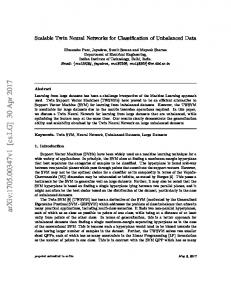
The shape of the hyper-ellipsoid is controlled by the distribution of the M nearest neighbors of the opposite class of the sample data si. We use Figure 1 and the three examples in Figure 2 to analyze the relationship between the distribution of the data samples in the feature space and the Gaussian CPS. In each example in Figure 2, we have one sample data illustrated in blue color, and its two nearest neighbors of opposite class marked as neighbor 1 and neighbor 2 illustrated in RED. One hundred new data samples were generated by the procedure described above and are represented by green “x”’s in all examples.
2
Neighbor 1
Sample 1
0
-2
-4 -8
-6
-4
-2
0
2
4
6
8
(b) 1
Sample 1
0.9
Neighbor 2 0.8 0.7 0.6
y
0.5 0.4 0.3 0.2
Neighbor 1 0
0.2
0.4
0.6
(c)
0.8
1
1.2
x
Figure 2. Three examples of different Gaussian CPS generated by different distributions of sample points.
1.4
It is clear that the newly generated data samples form an ellipse centered at the selected data sample. The principal axes are proportional to the two eigenvalues. In both Figure 2(a) and (b), the two nearest neighbors of the are located in the same direction, and the resulting ellipse is long and narrow. In both Figure 1 and Figure 2(c), the two nearest neighbors of each data sample are located in different directions in the feature space, more than 90o apart, the resulting ellipses are more like a circle, which means that the two eigenvalues in each example have very close values. Table 1 illustrates the eigenvalues, eigenvectors and the Euclidean distances between every sample data to its nearest neighbors. The characteristics of the eigenvalues and eigenvectors of the CPS are summarized as follows. 1. According to its definition, the first eigenvalue λ0 is a monotonically increasing function of the distance between sample data and its nearest neighbor of the opposite class. This is verified by our experiment result shown in Table 1. 2. If the nearest neighbors are located in the same orientation with respect to the sample point, the CPS ellipsoid is long in the principal axis but narrow at the others, and the new data samples have high density in the ellipse. In Figure 2 (a), the two nearest neighbors are close and at the same direction with respect to the sample data, and in (b), the two nearest neighbors are in the
same direction but quite apart. However the two CPS’s in Figure 2(a) and (b) are similar in shape, and the new data samples have high density in the both ellipses. 3. If the neighboring samples are far away from one another in terms of direction with respect to the sample data, the corresponding principal axes in the Gaussian CPS should be similar in lengths and the CPS is more like a circle. Both Figure 1 and Figure 2(c) along with Table 1 show this property of CPS. Quantitatively, this property can be measured by the ratio of λi i =0, 1. The difference between eigenvalues can help us to understand the distribution of the samples of the opposite class. For example, if λ0 is much larger than all of the other eigenvalues λi (I=1,2,…M-1), most of the data samples of the opposite class concentrate in the direction of the eigenvector corresponding to λ0 . If all of the M eigenvalues are very close to each other, the samples of the opposite class distribute evenly (to some extent) in a hypersphere around the sample. These properties of eigenvalues and the corresponding CPS ellipsoid are used to guide our training of neural networks.
d0
Figure 1 0.1211 0.0049
Figure 2(a) 0.9727 0.0393
Figure 2(b) 0.224 0.00906
Figure 2(c) 0.26 0.0105
E0 d1
[0.2873, -0.9578] T 0.3600 0.01336
[-0.6438, 0.7652] T 1.10269 0.000059
[-0.873, 0.488] T 0.933 0.000045
[-0.1961, -0.9806] T 0.6678 0.0228
λ0
λ1
[-0.9578, -0.2873] T [0.7652, 0.6438] T [0.488, 0.873] T [-0.9806, 0.1961]T E1 Table l The Euclidean distances di, eigenvectors, qi, eigenvalues, λi for i = 0, 1 of the examples shown in Figure 1 and 2.
3. Neural Learning from unbalanced training data This section describes the neural learning method that utilizes the Gaussian CPS distribution described in the last section. We attempt to train a neural network to learn the classification features
from the data samples of a minority class in the training set and to make more favorable decisions to the minority class. For the convenience of description, we referred to the two classes of data as minority and majority classes respectively. In many applications, if error is inevitable, a neural network is expected to err on one particular class
rather than the other. For example, in the classification of good/defect products in a manufacturing line, if a product is classified as a defect, it will be checked and repaired if necessary. Therefore, it is better to misclassify good products as defect rather than the other opposite type of error. Lu et al[1998] showed that in the case of unbalanced, noisy training data samples, multilayered backpropagation network(BP), Radial-Basis Function(RBF) and FUZZY ARTMAP all ignore the minority class, namely minority data samples are often misclassified. The algorithm we investigated was to generate new minority data samples near the classification boundary using the Gaussian CPS and add these new data samples to the training data. The neural networks trained on this set should make more favorable decision to the minority class with the minimization of misclassification of the majority class and have increased generalization capability. For every data sample s of the minority class in the training set, we attempt to generate p new data samples around s subject to its local Gaussian distribution of the opposite class. Let us assume the input vector is M dimensional. The noise modeling algorithm first finds the M data samples of the majority class that are closest to s, t1, t2, …, tM, from which we construct the MxM covariance matrix of the Gaussian probability density function described in the last section., and obtain M eigenvalues of the covariance matrix λ0 , λ1 , ..
λM −1 . We need to be cautious about generating new noise samples. If we generate unnecessary ones, we may weaken the classification capability of the neural network on the majority class. For example, if λ0 is large, it implies that s is quite apart from the majority class, and a neural network may easily learn the classification boundary around s. If we artificially generate more minority samples, we may force the trained neural network to make more classification error on the majority class than necessary. The noise modeling algorithm generates new data samples only at the locations where it is difficult to differentiate minority data samples from
the majority samples, and adding noisy random vectors does not affect too many majority samples. Based on the properties of Gaussian CPS, we developed the following rules. Let ρ1 and ρ 2 , the number of majority and minority samples falling within the hyper bounding box R of sample data s and s, t1, t2, …, tM respectively. Specifically, R is equal to ||s-t1||x||s-t2||x…||s-tM||. Rule1: If ρ1 , the density of majority class samples around s, is large, do not generate noisy data around s. Rule2: If ρ 2 , the density of minority class samples around s, is small, do not generate noisy data around s. Rule3: If λ0 , the 1st eigenvalue of Gaussian covariance matrix, is large, do not generate noisy data around s. For a minority data sample s, only if s does not satisfy any of the three rules, the noise modeling algorithm will generate p new data samples around s. The value p can be determined based on the ratio of the number of data samples in the majority and the minority class. Another important issue is to limit the noise random vectors in the hyper bounding box R. As we discussed in the last section that the random vectors fall within the CPS ellipsoid with the probability of v. However with the probability of 1-v, the new random vectors may fall outside the Gaussian CPS. Furthermore, the CPS ellipsoid may exceed the hyper bounding box R due to the symmetry of Gaussian distribution. Since we have no knowledge of what beyond these data samples, the noise modeling algorithm discard the new noise data samples generated beyond the hyper bounding box(see Figure 3). Therefore, the noise modeling algorithm accepts a random vector as a noise data sample only it belongs to the conjuncture of the rectangular and the ellipse(see Figure 3, where the rectangular is the bounding box equal to ||s-t 1||x||st2||.)
1 0.9 0.8 0.7
y
0.6 0.5 0.4 0.3 0.2
0
0.2
0.4
0.6
0.8
1
1.2
x Figure 3. Only the data samples that are within the conjuncture of the bounding box and the ellipse are accepted as new training data samples.
4. Experiments and Performances In this study, we conducted neural training using the noise modeling algorithm on a BP neural network[Rummelhar and McClelland, 1986] of three layers and a FUZZY ARTMAP neural network. The BP neural network has nodes 5-4-41, Momentum =0.90, Tanh function, and epoch size=16. A FUZZY ARTMAP network consists of two interconnected layers of neurons, F1 and F2. The input leads to activity in the feature detector neurons in F1, which is also called short-term memory activity. The short-term activity passes through connections to the neurons in F2. Each F2 neuron adds together its input from all the F1 neurons and generates an output. A measure will be taken over all the neurons in F2 and the output of one neuron will be selected as the system output, i.e. Winner-take-all. A major characteristic of a FUZZY ARTMAP network is that it allows a topdown feedback from F2 to reinforce the activity in F1. A learning algorithm of an FUZZY ARTMAP network is to determine wij , the top-down weight from winning node j in the F2 layer to a node i in the F1 layer, and z ji , the corresponding bottom-up weight. The detail of the learning algorithm can be found in[Carpenter et al, 1992; Lu et al, 1998]. The data used in the experiments are the vehicle test data acquired at the end-of-assembly
lines in the Ford Motor Company. The two neural networks are trained to classify whether a given vehicle is “good” or “bad” using input vectors in five dimensions. Since new vehicles manufactured by Ford Motor Company are mostly in the “good” class, the data samples in both the training set and test set are unevenly distributed. The data sets used in our study were downloaded directly from assembly plants in the Ford Motor Company. To illustrate the algorithm, we particularly chose the data samples from one particular vehicle model that contains high level of noise. We randomly separate the entire data samples into training and test with the ratio of 2:1. One way to estimate the noise level in a data set is to count the number of the opposite class samples within the hyper-bounding box of a given class. In the training set, we have total 727 good vehicle samples and 136 bad vehicle samples. We found that 96% good data samples are inside the hyper bounding box of bad vehicle class, and 88% of bad data samples are within the hyper bounding box of good vehicle class. In the test set, we have 356 good vehicle samples and 121 bad vehicle samples. We found that 93.3% of good vehicle samples are within the bad vehicle hyper bounding box and 85.7% bad vehicle samples are within the good vehicle hyper-bounding box. It can be interpreted as follows. In the training set, if we want to classify bad vehicles 100% correctly, we may be able to classify correctly only 4% of good vehicles; if we want to classify good vehicles 100% correctly, we may be able to classify correctly only 12% of bad vehicles. Similarly in the test set, , if we want to classify bad vehicles 100% correctly, we may be able to classify correctly only 6.7% of good vehicles; if we want to classify good vehicles 100% correctly, we may classify correctly only 14.3% of bad vehicles. These figures can be used as the performance metrics for a classifier: a neural network must give better performance than these figures. The experiment results of the two neural networks are shown in Table 2. The first experiment was conducted on the original training and test set. As we see from the first entry in Table 2 that the BP neural network was not at all capable of learning the features of the minority class from the training set, and as a result, the BP network fail
to classify any bad vehicles in either the training nor the test set. The FUZZY ARTMAP was better than the BP at learning the minority class features. It has achieved much better performance than the BP network on the minority class in both the training and the test data. The second experiment was conducted on the new training set obtained by duplicating every bad vehicle sample in the original training set 10 times and adding the newly generated ones to the training set. The BP network was able to classified a few of the minority class samples with the price of misclassifying a large number of good vehicle samples. FUZZY ARTMAP did not learn more about the minority class on this set of training data. Instead its performance on the minority class in the test set has dropped from the first experiment, even though its performance on the training data was very good. The third experiment was conducted on the new training data set generated using the noise modeling algorithm described in this paper. In the implementation, if the Gaussian CPS of each selected bad samples contained less than three good vehicle samples and more than one bad vehicle samples, then the noise modeling algorithm would generate ten random data samples around each of the selected bad vehicles were generated and added to the training set. The result of this experiment showed that both the BP network and the FUZZY ARTMAP network were able to learn from this new set of training data the classification feature of the minority class, and both gave much better classification capability on the minority class. The improvement of classification performance of the BP network is particularly interesting. While trained on the original training set, the BP network fail to classify any bad vehicles. After the training on the new training data, the BP network was able to classify more than 66% of bad vehicles on the training data and more than 45% on the test set, which is comparable to the FUZZY ARTMAP network. The FUZZY ARTMAP has in general better capability of learning the minority class features than the BP network as shown in the first two experiments. When the FUZZY ARTMAP network was trained on the new data set generated by the noise modeling algorithm, it gave better performance not only on the minority class but also on the majority class.
5. Conclusion We have presented an algorithm, noise modeling algorithm, for training a neural network to learn the classification features from unbalanced data samples. The algorithm was developed based on the Gaussian CPS theory to generate random noise over the classification boundary for a given training set with the aim of increasing classification features of a given class and the capability of generalization for the neural networks. We showed through experimental results that the noise modeling algorithm is effective in the training of both BP and FUZZY ARTMAP neural networks. We speculate that the algorithm can be extrapolated to the general classification problem of P classes within which the p classes are to be emphasized, where p < P. By generating noise data samples along the classification boundaries for these p classes using the noise modeling algorithm, the trained neural network would have increased classification capability and generalization ability over the p classes. 5. Acknowledgments This work is supported in part by a Grant from NSF DMII. 6. References [Carpenter et al, 1992;] G. A. Carpenter, S. Grossberg and N. Markuzon, et al., Fuzzy ARTMAP: An adaptive resonance architecture for incremental learning of ananlog maps, IJCNN June 1992, pp.309-314. [Dagli, 1992] Artificial Neural Networks for Intelligent Manufacturing, Edited by Cihan H. Dagli, 1992. [Kosko, 1992] Bart Kosko, Neural networks and fuzzy systems: A dynamical systems approach to machine intelligence, Prentice-Hall, 1992. [Lu et al 1998] Yi Lu, Hong Guo, and Lee Feldkamp, “Robust Neural Learning From Unbalanced Data Samples, IEEE IJCNN, 1998. [Mackay, 1991] David Mackay, Bayesian methods for adaptive models, Ph.D thesis, CIT, 1991.
[Musavi et al 1994] M. T. Musavi, K. H. Chan, D. M. Hummels, and K. Kalantri, “On the Generalization ability of Neural Network classifiers,” IEEE Transaction on Pattern Analysis and Machine Intelligence, Vol. 16, no. 6, pp. 659663, June 1994.
Data sets Original Training set Duplicate 10 Training data generated by the Constrained Gaussian CPS algorithm
[Rubinstein 1981] R. Y. Rubinstein, Simulation and the Monte Carlo method, John Wiley & Sons, 1981 [Rummelhar and McClelland, 1986] D.E. Rummelhart and J. L.McClelland. Parallel distributed processing: Explorations in the microstructure of cognition, vol 1: Foundations. MIT press, Cambridage, MA, 1986.
BP network: correctly classification rate Training set result Test set result Good vehicles: 100% Good vehicles: 100% Bad vehicles: 0% Bad vehicles: 0% Good vehicles: 45.94% Good vehicles: 48.31% Bad vehicles: 28.67%, Bad vehicles: 32.47% Good vehicles: 48.56% Good vehicles: 48.88% Bad vehicles: 66.77% Bad vehicles: 45.45%
Table 2. Experiment results of BP and FUZZY ARTMAP.
FUZZY ARTMAP: correctly classification rate Training set result Test set result Good vehicles: 87.3% Good vehicles: 69.66% Bad vehicles: 91.91%, Bad vehicles: 45.45% Good vehicles: 90.51% Good vehicles: 75.28% Bad vehicles: 94.12% Bad vehicles: 41.56% Good vehicles: 88.72% Good vehicles: 71.91% Bad vehicles: 94.25% Bad vehicles: 48.05%