Graphs with Obstacle Number Greater than One

Journal of Graph Algorithms and Applications http://jgaa.info/ vol. 0, no. 0, pp. 0–0 (0) DOI:

Graphs with Obstacle Number Greater than One Leah Wrenn Berman 1 Glenn G. Chappell 2 Jill R. Faudree 1 John Gimbel 1 Chris Hartman 2 Gordon I. Williams 1 1

Department of Mathematics & Statistics University of Alaska Fairbanks, Fairbanks, Alaska, USA 2 Department of Computer Science University of Alaska Fairbanks, Fairbanks, Alaska, USA

Abstract An obstacle representation of a graph G is a straight-line drawing of G in the plane, together with a collection of connected subsets of the plane, called obstacles, that block all non-edges of G while not blocking any edges of G. The obstacle number obs(G) is the least number of obstacles required to represent G. We study the structure of graphs with obstacle number greater than one. We show that the icosahedron has obstacle number 2, thus answering a question of Alpert, Koch, & Laison asking whether all planar graphs have obstacle number at most 1. We also show that the 1-skeleta of two related polyhedra, the gyroelongated 4-bipyramid and the gyroelongated 6bipyramid, have obstacle number 2. The order of the former graph is 10, which is also the order of the smallest known graph with obstacle number 2, making this the smallest known planar graph with obstacle number 2. Our methods involve instances of the Satisfiability problem; we make use of various “SAT solvers” in order to produce computer-assisted proofs.

1

Introduction

All graphs will be finite, simple, and undirected. Following Alpert, Koch, & Laison [2], we define an obstacle representation of a graph G to be a straightline drawing of G in the plane, together with a collection of connected subsets of the plane, called obstacles, such that no obstacle meets the drawing of G, while every non-edge of G is blocked by at least one obstacle. By non-edge, we mean a pair of distinct vertices a, b of G where ab is not an edge of G. A non-edge ab is blocked by an obstacle if the line segment joining a and b intersects the obstacle. The least number of obstacles required to represent G is the obstacle number of G, denoted obs(G). For clarity, we will sometimes refer to this as the ordinary obstacle number. The study of the obstacle number per se was initiated by Alpert, Koch, & Laison [2]. These parameters have since been investigated by 0

others [5, 7, 11, 12, 13, 14]. Determining whether obs(G) ≤ k for a given k is not in NP, shown by Johnson and Sarı¨oz [7]. Alpert, Koch, & Laison [2, Thm. 2] showed that there exist graphs with arbitrarily high obstacle number and asked [2, p. 229] for the smallest order of a graph with obstacle number greater than 1. They proved [2, Thm. 4] that the ∗ ∗ has obstacle number 2, where Ka,b (with a ≤ b) denotes the graph graph K5,7 obtained by removing a matching of size a from the complete bipartite graph Ka,b . Pach & Sarı¨ oz [14, Thm. 2.1] found a smaller example of a graph with ∗ obstacle number 2; in particular, they showed obs(K5,5 ) = 2. In an obstacle representation of a graph G, an outside obstacle is an obstacle that is contained in the unbounded component of the complement of the drawing of G. Any other obstacle is an interior obstacle. We define the outside obstacle number of G to be the least number of obstacles required to represent G, such that one of the obstacles is an outside obstacle—or zero if G has obstacle number zero. We denote the outside obstacle number of G by obsout (G). Clearly we have obs(G) ≤ obsout (G) ≤ obs(G) + 1 for every graph G. Alpert, Koch, & Laison [2, p. 231] asked whether every planar graph has obstacle number at most 1 (also see a series of questions in the Open Problem Garden [6]). They further asked for the obstacle numbers of the icosahedron and the dodecahedron. In Section 2, we develop tools for determining the obstacle numbers of particular graphs, and we use them to address these questions. In particular, we show that the obstacle number of the dodecahedron is 1, while the obstacle number of the icosahedron is 2. In addition, we show that the obstacle numbers of the 1-skeleta of the gyroelongated 4-bipyramid and the gyroelongated 4-bipyramid are each 2. The former is a planar graph of order 10; this is the first example of a planar graph with obstacle number greater than 1, and it is the smallest known example of such a graph. We conclude this section with an easy observation, which we will make use of throughout the remainder of this paper. Observation 1 Given an obstacle representation of a graph G, we can perturb all vertices an arbitrarily small distance to obtain an essentially equivalent obstacle representation in which no three vertices are collinear. Because of the above observation, we will generally assume that our obstacle representations have the property that no three vertices are collinear. Lest there be any confusion, only obstacles block edges; vertices do not. So the above observation has no impact on the definition of obstacle number.

2

Obstacle Number and Satisfiability

We now begin our development of tools for explicitly determining the obstacle number of a particular graph. Our ideas are based on the Satisfiability Problem (SAT). For each graph G, we construct a SAT instance encoding necessary conditions for the existence of an obstacle representation using a single obstacle. Thus, if we can show 1

that the instance is not satisfiable, then we know that obs(G) ≥ 2. There are a number of freely available, high-quality implementations of algorithms to determine satisfiability of a SAT instance. Using these, we will construct computer-aided proofs that obs(G) ≥ 2 for various planar graphs. For a, b, and c ∈ R2 , we say that abc is a clockwise triple if a, b, and c appear in clockwise order. We similarly define counter-clockwise triple. Note that for a triple abc, exactly one of the following is true: abc is clockwise, abc is counter-clockwise, or a, b, and c are collinear. For each triple abc, we introduce a Boolean variable xabc representing the statement that abc is a clockwise triple. By Observation 1 we may assume that no three vertices are collinear, so ¬xabc represents the statement that abc is a counter-clockwise triple. The following two lemmas give properties that hold for all point arrangements in the plane. Lemma 1 (4-Point Rule) Let a, b, c, and d be distinct points in R2 . If abc, acd, and adb are clockwise triples, then bcd must also be a clockwise triple. Proof: The 4-Point Rule is equivalent to what D. Knuth called the interiority property of triples of points; see Knuth [9, p. 4, Axiom 4].  In a SAT instance, the 4-point rule is represented by the clause ¬xabc ∨ ¬xacd ∨ ¬xadb ∨ xbcd .

(1)

Lemma 2 (5-Point Rule) Let a, b, c, d, and e be distinct points in R2 . If abc, acd, ade, and abe are clockwise triples, then either (i) both abd and ace are clockwise triples, or (ii) both abd and ace are counter-clockwise triples. Proof: This is equivalent to what D. Knuth called the transitivity property of triples of points; see Knuth [9, p. 4, Axiom 5].  In a SAT instance, the 5-Point Rule is represented by the following two clauses: ¬xabc ∨ ¬xacd ∨ ¬xade ∨ ¬xabe ∨ xabd ∨ ¬xace ;

(2)

¬xabc ∨ ¬xacd ∨ ¬xade ∨ ¬xabe ∨ ¬xabd ∨ xace .

(3)

Our SAT instance includes clauses from the 4-Point Rule corresponding to clause (1) for every set of 4 vertices of our graph, and every permutation of these 4 vertices. It also includes clauses from the 5-Point Rule corresponding to clauses (2) and (3) for every set of 5 vertices of our graph, and every permutation of these 5 vertices. Note that there are six ways to say vertices a, b, and c lie in clockwise order. When we construct our SAT instance, we may choose one of the variables from among 2

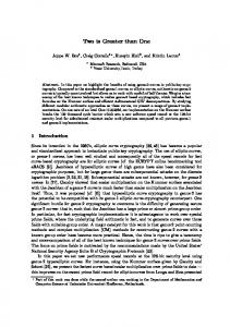
{xabc , xbca , xcab , xbac , xacb , xcba } as the canonical variable; we represent the other five using either the canonical variable or its negation, as appropriate. Additionally, the actions of even permutations of {b, c, d} on clauses (1) and (2) result in statements equivalent to the original; likewise an even permutation of {c, d, e} does not alter clause (3). This reduces the number of clauses required
by a factor of
3. Thus, for an n-vertex graph, our SAT
instance in-
cludes n4 ·4!/3 = 8 n4 clauses based on the 4-Point Rule and 2 n5 ·5!/3 = 80 n5 clauses based on the 5-Point Rule. In the next lemma, given distinct points a and b, we denote the two closed ← → + − + halfplanes determined by line ab as Hab and Hab , where Hab contains all points ← → y such that either y is on line ab or aby is oriented clockwise. An ab-key-path with respect to cd, denoted Pab (cd), is a path from a to b that does not cross ← → the line cd ; that is, a path in G from a to b that is entirely contained in one of + − the closed halfplanes Hcd or Hcd ; see Figure 1.

b P1

c

a P2

d

Figure 1: An ab-key-path with respect to cd, denoted Pab (cd), is a path from a ↔

to b that does not cross the line cd. The path P1 (blue) is an ab-key-path with respect to cd, but the path P2 (red) is not.

Lemma 3 Suppose we are given an obstacle representation of a graph G that uses at most one obstacle. Then, for each non-edge ab, and for each non-edge cd 6= ab (ab and cd may share one vertex), there exists a halfplane Hab (cd) ∈ + − {Hab , Hab } such that if Pab (cd) is an ab-key-path with respect to cd, then some internal vertex of Pab (cd) lies in the interior of Hab (cd). Proof: Choose any non-edge ab, and then choose a second non-edge cd distinct ← → ← → from ab. Perturbing slightly if necessary, we assume that ab 6= cd as well (see Observation 1). Suppose for a contradiction that there exist two distinct ab paths P1 and P2 in G, both ab-key-paths with respect to cd, that lie in different ← → closed halfplanes determined by ab . Without loss of generality, we may assume + − that P1 ⊆ Hab and P2 ⊆ Hab . 3

+ − Now, each of P1 , P2 is contained in one of the two halfplanes Hcd , Hcd , because they are key-paths with respect to cd. Since P1 and P2 have common endpoints, namely a and b, we see that P1 and P2 must be contained in the ← → same halfplane determined by cd . Therefore P1 ∪ P2 forms a closed path in the plane; the open line segment ab lies in one component of the complement of this closed path; while the open line segment cd lies in a different component. Since G has only one obstacle, it is impossible for both segments to be blocked, a contradiction. 

Given a graph G, we can use Lemmas 1 (the 4-Point rule), 2 (the 5-Point Rule), and 3 to create a SAT instance encoding necessary conditions for the existence of an obstacle representation of G using at most 1 obstacle. If this SAT instance is not satisfiable, then we may conclude that graph G requires at least two obstacles, that is, that obs(G) > 1. If the SAT instance is satisfiable, we can not conclude anything about the obstacle number of G. We illustrate the encoding of Lemma 3 in terms of SAT clauses by showing how to encode statements about a particular path. Let ab and cd be distinct non-edges. Let a, s, t, . . . , u, b be the sequence of vertices in some ab-path P (not necessarily a key-path), where vertices a, b are not adjacent (so that ab is a non-edge). We introduce a new variable kP (cd) to represent the statement that P is an ab-key-path with respect to cd. If all vertices v of P , with v 6∈ {c, d}, produce triangles cdv having the same orientation, then P is a key-path. This is encoded by the following two clauses, where we omit literals involving triples in which vertex c or d appears twice: xcda ∨ xcds ∨ xcdt ∨ · · · ∨ xcdu ∨ xcdb ∨ kP (cd) ;

(4)

¬xcda ∨ ¬xcds ∨ ¬xcdt ∨ · · · ∨ ¬xcdu ∨ ¬xcdb ∨ kP (cd) .

(5)

Next we encode the statement that given this ab and cd we can find a “special” side of ab so that every ab-key-path with respect to cd has an internal vertex lying on the special side of ab. The special side is encoded in another variable, sab,cd . We canonically choose that sab,cd represents the statement that + the special halfplane is Hab ; thus ¬sab,cd represents the statement that the spe− cial halfplane is Hab . Note that the special side of ab depends on the choice of non-edge cd. The following clauses encode the desired statement: ¬kP (cd) ∨ ¬sab,cd ∨ xabs ∨ xabt ∨ · · · ∨ xabu ;

(6)

¬kP (cd) ∨ sab,cd ∨ ¬xabs ∨ ¬xabt ∨ · · · ∨ ¬xabu .

(7)

Observation 2 Let G be a graph. If obs(G) ≤ 1, then the SAT instance consisting of all clauses of the forms (1)–(7), using canonical variables, is satisfiable. It is important to note that if our SAT instance is not satisfiable, then we are guaranteed that it is impossible to draw the graph using a single obstacle; i.e., obs(G) ≥ 2. However, if the SAT instance is satisfiable, then it does not 4

follow that obs(G) ≤ 1; satisfiability is a necessary but not sufficient condition for obs(G) ≤ 1. Using these ideas, we can determine the exact value of the obstacle number for the icosahedron and some similar graphs. Following Johnson [8], for n ≥ 3 we define the gyroelongated n-bipyramid to be a convex polyhedron formed by adding pyramids to the top and bottom base of the n-antiprism; see Figure 2. The gyroelongated square bipyramid, when constructed using equilateral triangles, is also known as the Johnson solid J17 . The gyroelongated pentagonal bipyramid, again when constructed of equilateral triangles, is the regular icosahedron. We denote the skeleton of the gyroelongated n-bipyramid by Xn . We also refer to X5 as I, since it is the icosahedron. The graph Xn can be constructed as two disjoint n-wheels, connected by a 2n-cycle that alternates between vertices of the wheel boundaries taken cyclically. Figures 2, 3, 4, and 6 show gyroelongated n-bipyramids for various values of n, while Figure 5 illustrates the general case.

3

2 3

2 4

3

2

3 1

3

4

1

4

(a) X3

1 2

1

(b) X4

2

1

5

3

4 5

2 1

(c) X5 = I

Figure 2: Gyroelongated n-bipyramid skeleta; the antiprisms are highlighted in black and green, while the pyramids erected on the bases are shown in blue.

In each of these figures, the wheel boundaries are labeled with consecutive integers and are shown in green, the spokes of the wheel in blue, and the connecting cycle in black; the cycle connecting the two wheel boundaries corresponds to the sequence of labeled vertices 1, 1, 2, 2, . . . , n, n. Non-edges are shown with thin gray or pink lines. Proposition 3 All of the following hold. 1. obs(X4 ) = obsout (X4 ) = 2. 2. obs(I) = obsout (I) = 2. 3. obs(X6 ) = obsout (X6 ) = 2. Proof: The lower bounds were found using a computer. We create a SAT instance as described above, using clauses representing the 4-Point Rule, the 5Point Rule, and the statement of Lemma 3. See [4] for software to generate the 5

1

2

2

1

3

5

4

4

5

3

(a)

(b)

Figure 3: Two 2-obstacle embeddings of the icosahedron. The interior obstacle is highlighted in pale magenta, and non-edges blocked by that obstacle are shown with thin magenta lines. The other obstacle is the outside obstacle, and non-edges blocked by that obstacle are shown with thin gray lines.

1

2

2

1

2

1 2

3

4

1

3

6 5

4 5

4

4

6

3

(a) X4

3

(b) X6

Figure 4: Two-obstacle embeddings of gyroelongated n-bipyramids; n = 4, 6.

6

1

2

2

1

3

n n-1 4 5

5

n-1 4 n

3

Figure 5: A two-obstacle embedding of a gyroelogated n-bipyramid.

(a) The gyroelongated 3-bipyramid X3

(b) A one-obstacle embedding of X3 .

Figure 6: obs(X3 ) = 1.

7

SAT instances. For each graph, a standard SAT solver (we used MiniSat [10], PicoSAT [3], and zChaff [15]) indicates that the SAT instance is not satisfiable. For the upper bounds, we exhibit an obstacle representation of each graph using two obstacles, one of which is an outside obstacle. Figure 3 shows drawings of the icosahedron, while Figure 4 shows drawings of X4 and X6 .  Proposition 3 answers in the negative a question of Alpert, Koch, & Laison [2, p. 231] asking whether every planar graph has obstacle number at most 1. Part (2) of that proposition also answers a related question of Alpert, Koch, & Laison asking for the obstacle number of the icosahedron. Note also that the graph X4 , mentioned in part (1) of Proposition 3, has order 10. This is thus the second known example of a graph of order 10 with ∗ obstacle number 2 (the first being K5,5 , shown to have obstacle number 2 by Pach & Sarı¨ oz [14, Thm. 2.1]). But unlike the Pach-Sarı¨oz example, graph X4 is planar. We do not know whether there is any planar graph—or, indeed, any graph at all—of smaller order that has obstacle number 2. The gyroelongated 3-bipyramid can be drawn with a single outside obstacle; see Figure 6. As for the gyroelongated n-bipyramid for n ≥ 6, we conjecture that they all have obstacle number 2. Conjecture 4 If n ≥ 4, then obs(Xn ) = obsout (Xn ) = 2. If we are interested in bounding only the outside obstacle number, we can replace Lemma 3 with the following: Lemma 4 Suppose we are given an obstacle representation of a graph G using no interior obstacles. Let ab be a non-edge of G. Then there exists a half-plane ← → H determined by the line ab such that, for each ab-path P in G, some internal vertex of P lies in H. We can develop SAT clauses based on the above lemma as before. Specifically, Lemma 4 implies that, for each pair of nonadjacent vertices a, b of G, one of the two half-planes determined by segment ab is “special”: this halfplane contains at least one internal vertex from each ab-path in G. We create a Boolean new variable sab representing the statement that the special half-plane is that containing points p such that abp is a clockwise triple. Let a, s, t, . . . , u, b be the sequence of vertices in some ab-path P . Then the following clauses represent the statement of Lemma 4 for P : ¬sab ∨ xabs ∨ xabt ∨ · · · ∨ xabu

(8)

sab ∨ ¬xabs ∨ ¬xabt ∨ · · · ∨ ¬xabu

(9)

As with the x variables, we choose one of sab and sba to be the canonical variable, and we represent the other by its negation. Observation 5 Let G be a graph. If obsout (G) ≤ 1, then the SAT instance consisting of all clauses of the forms (1)–(3), (8), and (9)—using canonical variables, as discussed—is satisfiable. 8

Compare the earlier SAT instance of Observation 2 with that of Observataion 5. Clauses (4)–(7), which are generated for each ordered pair of distinct non-edges, are replaced by clauses (8) and (9), generated only for each nonedge. This smaller SAT instance may allow for computations involving larger graphs. However, we have not (yet) obtained any additional results from this SAT instance. Alpert, Koch, & Laison [2, p. 229] asked (using different terminology) whether every graph G with obs(G) = 1 also has obsout (G) = 1. We ask a more general question. Question 6 Is it true that obs(G) = obsout (G) for every graph G? We conjecture that the answer is yes. Alpert, Koch, & Laison [2, p. 231] asked for the obstacle number of the dodecahedron. We answer this question as follows. Proposition 7 Let D be the dodecahedron. Then obs(D) = obsout (D) = 1. Proof: Figure 7 shows an obstacle representation of the dodecahedron, using a single outside obstacle. 

3

Open questions

There are several interesting open questions related to obstacle numbers of graphs with small numbers of vertices. In general, little is known about the least order of a graph with any particular obstacle number or outside obstacle number. Question 8 What is the minimum order of a graph G with obsout (G) = 2? With obs(G) = 2? With obsout (G) or obs(G) > 2? It is not difficult to show that all graphs G with order at most 5 have obsout (G) ≤ 1, so for each of the above questions the answer must be at least ∗ 6. The drawing of K5,5 by Pach & Sari¨oz [14] and the drawing of the gyroelongated square bipyramid in Figure 4 show that both of these graphs have outside obstacle number 2, so the answer to the first two questions must lie between 6 and 10 inclusive. Question 9 What is the minimum order of a planar graph with obstacle number 2? The gyroelongated square bipyramid is a planar graph with order 10, so the minimum order is between 6 and 10. It is natural to ask whether there exists an upper bound on the obstacle numbers of planar graphs, and, if so, what it is. It seems likely that either there is no such upper bound, or else the maximum obstacle number of a planar graph is 2. We conjecture that the latter option holds. 9

F G

K

L

I H

E J

F E

B

J

G

A D

D

C I

P S

A

C

H

O

M N

B Q

R

Q S P

R

K

T T

M N

L

O

(a) A drawing of the dodecahedron

(b) An obstacle representation using a single outside obstacle.

Figure 7: A drawing of the dodecahedron, with useful edge-colorings, and an obstacle representation of the dodecahedron using a single outside obstacle (with corresponding edges and vertices).

10

Conjecture 10 If G is a planar graph, then obs(G) ≤ 2. We have found the above questions quite resistant to solution. Perhaps this is unsurprising since Johnson & Sarı¨oz [7] showed that computing the obstacle number of a plane graph is NP-hard. Two examples of graphs of order 10 with ∗ obstacle number 2 have been found, namely K5,5 and X4 ; none of smaller order are known. If we knew of a single graph of order 9 or less for which one of the SAT instances we construct is not satisfiable, then we could reduce our current bound of 10; however we have found no such graph. It seems plausible that an approach to answering the above questions would be a brute-force application of SAT instances to all graphs with order strictly less than 10. However, this naive approach has two flaws. First, there are a large number of graphs of order at most 9 (for example, there are 11117 connected graphs of order 8 and 261080 connected graphs of order 9 [1, Sequence A001349]), and there are significant time and computational issues involved in processing the SAT instances for all these graphs. Second, while non-satisfiability of the SAT instance for one of these graphs would imply that the corresponding (outside) obstacle number was strictly greater than 1, satisfiability of an instance does not imply any bound on the corresponding obstacle number. The solution of one of our SAT instances gives only a specification of clockwise/counter-clockwise orientation for each triple of points. This might not correspond to any actual point placement in the plane. Or it may correspond to many point placements. And even if one of these gives the desired obstacle representation, others may not; or none of them may. Furthermore, a single SAT instance can have exponentially many solutions, each of which may need to be checked, in order to find an obstacle representation. In any case, satisfiability provides us only with a starting point in the search for an obstacle representation; we know of no efficient, reliable technique for actually finding such a representation without human intervention and invention.

References [1] The On-Line Encyclopedia of Integer Sequences, 2013, http://oeis.org. [2] Hannah Alpert, Christina Koch, and Joshua D. Laison, Obstacle numbers of graphs, Discrete Comput. Geom. 44 (2010), no. 1, 223–244. MR 2639825 (2011g:05208) [3] A. Biere, PicoSAT essentials, Journal on Satisfiability, Boolean Modeling and Computation 4 (2008), 75–97. [4] Glenn G. Chappell, Software for computing SAT instances related to obstacle number, http://www.cs.uaf.edu/~chappell/papers/obstsoft. [5] Radoslav Fulek, Noushin Saeedi, and Deniz Sarı¨oz, Convex obstacle numbers of outerplanar graphs and bipartite permutation graphs, Thirty essays 11

on geometric graph theory, Springer, New York, 2013, pp. 249–261. MR 3205157 [6] Open Problem Garden, Obstacle number of planar graphs, http://www. openproblemgarden.org/op/obstacle_number_of_planar_graphs. [7] Matthew P. Johnson and Deniz Sarı¨oz, Representing a planar straight-line graph using few obstacles, Proc. 26th Canadian Conference on Computational Geometry (CCCG ’14), http://www.cccg.ca/proceedings/2014/papers/paper14.pdf, 2014. [8] Norman W. Johnson, Convex polyhedra with regular faces, Canad. J. Math. 18 (1966), 169–200. MR 0185507 [9] D. E. Knuth, Axioms and hulls, Lecture Notes in Computer Science, vol. 606, Springer-Verlag, Berlin, 1992. MR 1226891 [10] MiniSat, http://minisat.se. [11] Padmini Mukkamala, J´anos Pach, and D¨om¨ot¨or P´alv¨olgyi, Lower bounds on the obstacle number of graphs, Electron. J. Combin. 19 (2012), no. 2, Paper 32, 8. MR 2928647 [12] Padmini Mukkamala, J´anos Pach, and Deniz Sarı¨oz, Graphs with large obstacle numbers, Graph-theoretic concepts in computer science, Lecture Notes in Comput. Sci., vol. 6410, Springer, Berlin, 2010, pp. 292–303. MR 2765279 (2012e:05100) [13] J´ anos Pach and Deniz Sarı¨oz, Small (2,s)-colorable graphs without 1obstacle representations, ArXiV, http://arxiv.org/abs/1012.5907 (2010), Ancillary to “On the structure of graphs with low obstacle number”, Graphs and Combinatorics, Volume 27, Number 3. [14] J´ anos Pach and Deniz Sarı¨oz, On the structure of graphs with low obstacle number, Graphs Combin. 27 (2011), no. 3, 465–473. MR 2787431 (2012d:05268) [15] zChaff, http://www.princeton.edu/~chaff/zchaff.html.

12