Aug 25, 2010 - struct a discrete incremental model for bridge decks where the .... Infinity. Using the information in Table 2, a transition probability matrix can be ...
ERDC/CHL CHETN-IX-25 August 2010
Guide to the Development of a Deterioration Rate Curve Using Condition State Inspection Data by Guillermo A. Riveros and Elias Arredondo PURPOSE: The deterioration of elements of steel hydraulic structures (SHS) on our nation’s lock system is caused by combined effects of several complex phenomena: corrosion, cracking and fatigue, impact, and overloads. This Coastal and Hydraulics Engineering Technical Note presents a procedure for generating a deterioration rate curve when condition state inspection data are available. BACKGROUND: This Technical Note presents the procedure used for generating the deterioration curve presented in Riveros and Arredondo (2010). DERIVATION OF TRANSITION PROBABILITIES: Transition probability specifies the likelihood that the condition of an infrastructure facility will change from one state to another in a stipulated time period. Transitions are probabilistic in nature because of the uncertainty in predicting infrastructure deterioration from inspection data and the inherent stochasticity of the deterioration process. The most common method and the one easiest to use for determining the transition probabilities has been the linear regression method (Carnahan et al. 1987). It consists of separating the facilities into groups with similar deficiencies, material types, and other explanatory variables. Then, for each group a deterioration model is estimated by linear regression with the deterioration state as a dependent variable and age as the independent variable. The transition probability is then calculated. Madanat et al. (1995) used the Poisson regression model to calculate the transition probabilities of infrastructure facilities. This model provides a logical description for events that occur both randomly and independently over time. Madanat et al. used the Poisson regression model to construct a discrete incremental model for bridge decks where the dependent variables are the number of changes in the condition state in one inspection period. Since the available data containing condition states are limited for navigation structures, the development of a probabilistic method that can be updated as data become available is proposed. The method will be described and illustrated by generating synthetic data using a Weibull distribution and Latin hypercube simulation (LHS) as the sampling method, producing the final transition probability matrix and deterioration curve. The following assumptions are considered necessary concerning the collection and distribution of the actual data. 1. Data shall be collected for several different structures (or components).
Form Approved OMB No. 0704-0188
Report Documentation Page
Public reporting burden for the collection of information is estimated to average 1 hour per response, including the time for reviewing instructions, searching existing data sources, gathering and maintaining the data needed, and completing and reviewing the collection of information. Send comments regarding this burden estimate or any other aspect of this collection of information, including suggestions for reducing this burden, to Washington Headquarters Services, Directorate for Information Operations and Reports, 1215 Jefferson Davis Highway, Suite 1204, Arlington VA 22202-4302. Respondents should be aware that notwithstanding any other provision of law, no person shall be subject to a penalty for failing to comply with a collection of information if it does not display a currently valid OMB control number.
1. REPORT DATE
3. DATES COVERED 2. REPORT TYPE
AUG 2010
00-00-2010 to 00-00-2010
4. TITLE AND SUBTITLE
5a. CONTRACT NUMBER
Guide to the Development of a Deterioration Rate Curve Using Condition State Inspection Data
5b. GRANT NUMBER 5c. PROGRAM ELEMENT NUMBER
6. AUTHOR(S)
5d. PROJECT NUMBER 5e. TASK NUMBER 5f. WORK UNIT NUMBER
7. PERFORMING ORGANIZATION NAME(S) AND ADDRESS(ES)
U.S. Army Engineer Research and Development Center,3909 Halls Ferry Road,Vicksburg,MS,39180 9. SPONSORING/MONITORING AGENCY NAME(S) AND ADDRESS(ES)
8. PERFORMING ORGANIZATION REPORT NUMBER
10. SPONSOR/MONITOR’S ACRONYM(S) 11. SPONSOR/MONITOR’S REPORT NUMBER(S)
12. DISTRIBUTION/AVAILABILITY STATEMENT
Approved for public release; distribution unlimited 13. SUPPLEMENTARY NOTES 14. ABSTRACT
15. SUBJECT TERMS 16. SECURITY CLASSIFICATION OF: a. REPORT
b. ABSTRACT
c. THIS PAGE
unclassified
unclassified
unclassified
17. LIMITATION OF ABSTRACT
18. NUMBER OF PAGES
Same as Report (SAR)
12
19a. NAME OF RESPONSIBLE PERSON
Standard Form 298 (Rev. 8-98) Prescribed by ANSI Std Z39-18
ERDC/CHL CHETN-IX-25 August 2010
2. Data shall be collected at regular intervals (although it may be for a different group of structures at each interval). 3. Data shall be grouped by type of structure, location, waterways, climatic conditions, hydrostatic head, or some other criteria. 4. The data may have a normal, log-normal, or Weibull distribution. WEIBULL DISTRIBUTION: A Weibull distribution is most commonly used in reliability studies to help predict the lifetime of a device. Weibull analysis can be used to make predictions about a product’s life, compare the reliability of different products, or proactively predict when a product needs to be replaced. It is defined by the density function: x f x
1
e
x
(1)
where 0 ≤ x ≤ ∞ and α and β are both greater than zero. α is known as the characteristic life and is a measure of the scale, or spread, in the distribution of data. β is known as the shape parameter and indicates whether the deterioration rate is constant, increasing, or decreasing. Figure 1 shows the Weibull distribution with α = 0.2 and β = 0.4. The shape of the distribution curve changes with the values of the parameters. It can mimic other distributions such as lognormal and normal as shown in Figure 2. From the Weibull distribution parameters, the statistic parameters can be calculated. Equations 2, 3, and 4 show how to obtain the mean, median, and the variance as a function of α and β. Statistics Mean:
1
(2)
where Γ is the gamma function defined as n e x x n 1dx . 0
Median:
1n 2
1
2
(3)
ERDC/CHL CHETN-IX-25 August 2010
Weibull Distribution 30 25
f(x)
20 15 10 5 0 0.0
0.1
0.2
0.3
0.4
0.5
0.6
x Figure 1. Weibull distribution graph for α = 0.2, β = 0.4.
Weibull Distribution 2.00
f(x)
1.50
alpha=2, beta=0.5 alpha=3, beta=1.5
1.00
0.50
0.00 0.0
1.0
2.0
3.0
4.0
x
Figure 2. Weibull distribution mimicking other distributions.
3
5.0
ERDC/CHL CHETN-IX-25 August 2010
Variance:
2
2 1 2
1
2
(4)
Generating Weibull Distributed Random Numbers. Given a random number x drawn from a uniform distribution in the interval (0, 1), the number y has a Weibull distribution with parameters α and β. 1
y 1n x
(5)
A set of 25 random numbers, simulating condition ratings for 25 different structures, are generated by the LHS method. The process begins with the generation of 25 random numbers in the interval (0, 1) having a uniform distribution. For a uniform distribution, the Cumulative Distribution Function (CDF) is shown in Figure 3. Cumulative Distribution Function 1.00 0.90 0.80
Probability
0.70 0.60 0.50 0.40 0.30 0.20 0.10 0.00 0.00
0.10
0.20
0.30
0.40
0.50
0.60
0.70
Distribution Figure 3. Cumulative Distribution Function for a uniform distribution.
4
0.80
0.90
1.00
ERDC/CHL CHETN-IX-25 August 2010
The probability axis is divided into 25 equal segments, one segment for each value. Each segment represents 1/25 or 4 percent of the total probability. The first segment begins at 0 and ends at 0.04. Similarly, the second segment begins at 0.04 and ends at 0.08 and the nth segment begins at (n - 1)/25 and ends at n/25. Beginning with the first segment, a random number is generated within the range of the segment (0–0.04). For example, say the random number generated is 0.026344. Using this probability value, determine where it intersects the CDF curve and read the corresponding distribution value. Since this is a uniform distribution, the distribution value will be the same as the probability value. The transformation given by Equation 3 is applied to this value. To illustrate the procedure, the following values for the parameters are arbitrarily assigned (as data become available, these parameters can be calculated from the actual distribution) α = 20, β = 1.02. The result is y 1.02 ln 0.026344
1/ 20
1.088014
For the next segment, a random number is generated in the range 0.04 to 0.08. Say the random number generated is 0.046516. Applying the transformation results in the value: y 1.02 ln 0.046516
1/20
1.078804
This process is continued for all 25 simulations. Table 1 shows the results. Table 1. Results of a typical LHS simulation Simulation
x
y
Simulation
x
y
1
0.026344
1.088014
14
0.547430
0.994486
2
0.046516
1.078804
15
0.570050
0.991033
3
0.081322
1.068017
16
0.634426
0.980624
4
0.146766
1.053787
17
0.666647
0.974988
5
0.183902
1.047219
18
0.706491
0.967486
6
0.234242
1.039177
19
0.731436
0.962409
7
0.269452
1.033919
20
0.777029
0.952125
8
0.316732
1.027139
21
0.827824
0.938465
9
0.344843
1.023201
22
0.842100
0.934025
10
0.377016
1.018734
23
0.886355
0.917644
11
0.430842
1.011268
24
0.940449
0.887172
12
0.459083
1.007311
25
0.978199
0.842875
13
0.503773
1.000932
Additional sets of random numbers are generated at 5-year intervals. For each interval the median value is plotted in Figure 4.
5
ERDC/CHL CHETN-IX-25 August 2010
Deterioration (Weibull Distribution) Time (Years) 0
10
20
30
40
50
60
1
Condition State
2 Min Median Max
3
4
5 Figure 4. Graph of synthetic rating values with Weibull distribution.
With the synthetic data generated, the next step is to generate a transition probability matrix. This is done by considering the length of time between condition states. From Figure 4, it appears that somewhere around 30 years the condition state reaches a value of 2. By linear interpolation, using the values from Table 2, the actual value is found to be 29.937 years. So it is considered that condition 1 extends from year 0 to year 29.937. The time duration of each condition state was calculated from the data plotted in Figure 4 and is listed in Table 2. Table 2. Duration of Condition Ratings Year
Condition Rating
Years in This Condition
0.0000
1.00
29.9373
29.9373
2.00
15.0000
44.9373
3.00
8.4483
53.3856
4.00
6.5674
59.9530
5.00
Infinity
Using the information in Table 2, a transition probability matrix can be generated. The value in the last column was used to calculate the probability of changing from one condition to the next. The probability of change is calculated as the inverse of the number of years in the current
6
ERDC/CHL CHETN-IX-25 August 2010
condition. The resulting transition probability matrix and deterioration curve are shown in Table 3 and Figure 5, respectively. Table 3. Transition Probability Matrix Condition Rating
Years in Condition
Probability of Change
Probability of No Change
1
29.9373
0.033
0.967
2
15.0000
0.067
0.933
3
8.4483
0.118
0.882
4
6.5674
0.152
0.848
5
Infinity
0.000
1.000
Figure 5. Deterioration rate.
Generation of Deterioration Rate Curve with Existing Data. This section presents an example of how to generate a deterioration rate curve when condition state inspection data are available. The procedure uses data obtained from Agrawal et al. 2008.
These data will be used to generate a deterioration rate curve with the Sauser and Riveros (2009) system.
7
ERDC/CHL CHETN-IX-25 August 2010
The data are for four different types of elements: steel plate girders, steel rolled beams, weathering steel rolled beams, and weathering steel plate girders. The data were collected over a period of 117 years, 114 years, 36 years, and 35 years, respectively. The data represent the mean condition rating of multiple elements. A graph of the data is shown in Figure 6. The upward peaks in the data (improvements in the condition rating) are most likely the result of maintenance/repairs done to the elements. Synthetically generated Weibull distribution data are also shown in the graph.
Figure 6. New York Department of Transportation condition rating states.
The New York Department of Transportation data are based on a scale of 7 to 1 with 7 representing the best condition and 1 representing the worst condition. The Sauser and Riveros (2009) system is from 1 to 5 with 1 representing the best condition and 5 representing the worst condition. To adapt the New York Department of Transportation data to the Sauser and Riveros (2009) rating system, the data were first transposed to a 1 to 5 rating system (Figure 7). The 7 to 1 rating system was linearly scaled down to a 5 to 1 system and then inverted to a 1 to 5 system. After the data were transposed, the average rating of the four different types of elements was calculated and a linear regression of the average rating values was performed. The linear regression was performed to remove the upward peaks of the actual data. Other types of regression could also be used, but the data appear to best fit a straight line. The result is shown in Figure 8. Using the linear regression line as mean values, synthetic values were generated for condition ratings every 5 years. The generated values are shown in Figure 8.
8
ERDC/CHL CHETN-IX-25 August 2010
Figure 7.
New York Department of Transportation data averaged and transposed to Sauser and Riveros (2009) rating system.
Figure 8.
Synthetic condition rating values with normal distribution.
9
ERDC/CHL CHETN-IX-25 August 2010
For each 5-year interval, 25 synthetic values were generated. These values are represented by the vertical rows of dots in Figure 8. The LHS method was used for generating the synthetic rating values. A normal distribution was assumed. The mean was selected as the value generated from the linear regression line. The standard deviation was selected to give the values a range of one in the rating condition axis. For example, an examination of the values for age 20 years on the graph in Figure 8 shows that the range of the values extends from approximately condition 1 to condition 2 with a mean value of about 1.5. With the synthetic data generated, the next step was to generate a transition probability matrix. This was accomplished by considering the length of time between condition states. From Figure 8, it appears that somewhere around 37 years the condition state reaches a value of 2. By linear interpolation of the data, the actual value was found to be 37.151597 years. So it was considered that condition 1 extends from year 0 to year 37.151597. The time duration of each condition state was calculated and is listed in Table 4. Table 4. Duration of Condition Ratings for Synthetic Data Year
Condition Rating
Years in This Condition
0.000000
1
37.151597
37.151597
2
36.275493
73.427090
3
35.682399
109.109490
4
36.496349
145.605839
5
infinity
Using the information in Table 4, a transition probability matrix was generated. The value in the last column was used to calculate the probability of changing from one condition to the next. The probability of change was calculated as the inverse of the number of years in the current condition. The resulting transition probability matrix and deterioration curve are shown in Table 5 and Figure 9, respectively. Table 5. Transition Probability Matrix for Synthetic Data Condition Rating
Years in This Condition
Probability of Change
Probability of No Change
1
37.151597
0.027
0.973
2
36.275493
0.028
0.972
3
35.682399
0.028
0.972
4
36.496349
0.027
0.973
5
Infinity
0.000
1.000
CONCLUSIONS: The theory of the Markov chain is well developed and based on simple multiplications of matrices. The application of the Markov chain provides navigation structures managers a powerful and convenient tool for estimating structure service life. Service life prediction by Markov chain has the advantage over the statistical regression approach in that it can be used to estimate not only the average service life of navigation structures but also the service life of any individual structural component. Furthermore, the Markov chain prediction is
10
ERDC/CHL CHETN-IX-25 August 2010
Deterioration Rate (Markov Prediction Model) Time (years) 0
10
20
30
40
50
60
70
80
90
100
1
Rating (R)
2
3
4
5 Figure 9.
Deterioration rate.
based on the current condition and age of the structure; therefore, it is simple and can be updated by new information of condition states and structure age. However, it should be noted that this study was based on synthetic data and assumed that limited numbers of inspection reports with condition states are available. However, by utilizing the Latin hypercube analytical tools to generate random numbers based on a predefined distribution, it was possible to obtain realistic values to define the transition probability and therefore the deterioration curve. The procedure was also used with existing data for a combination of steel bridge plate girders, rolled beams, weathering rolled beams, and weathering plate girders and demonstrates a model that can be implemented and used efficiently with any navigation structures. ADDITIONAL INFORMATION: For additional information contact Dr. Guillermo A. Riveros, Information Technology Laboratory, U.S. Army Engineer Research and Development Center, 3909 Halls Ferry Road, Vicksburg, MS 39180 at 601-634-4476, or e-mail Guillermo.A.Riveros@ usace.army.mil. This effort was funded through the Navigation Systems Research Program. Program Manager is Charles Wiggins, phone 601-634-2471, e-mail Charles.E.Wiggins@usace. army.mil. This CHETN should be cited as follows:
Riveros, G. A., and E. Arredondo. 2010. Predicting deterioration of navigation steel hydraulic structures with Markov chain and Latin hypercube simulation. Coastal and Hydraulics Engineering Technical Note ERDC/CHL CHETN-IX-25. 11
ERDC/CHL CHETN-IX-25 August 2010
Vicksburg, MS: U.S. Army Engineer Research and Development Center. An electronic copy of this CHETN is available from http://chl.erdc.usace.army.mil/ chetn. REFERENCES Agrawal, A. K., A. Kawaguchi, and G. Qian. 2008. Bridge deterioration rates. Albany, NY: Transportation Infrastructure Research Consortium, New York State Department of Transportation. Carnahan, J. V., W. J. Davis, and M. Y. Shahin. 1987. Optimal maintenance decisions for pavement management. Journal of Transportation Engineering, ASCE , 113(5): 554-572. Madanat, S., R. Mishalani, and W. H. W. Ibrahim. 1995. Estimation of infrastructure transition probabilities from condition rating data. Journal of infrastructure systems 1(2): 120-125. Riveros, G. A., and E. Arredondo. 2010. Predicting deterioration of navigation steel hydraulic structures with Markov chain and Latin hypercube simulation. Coastal and Hydraulics Engineering Technical Note, ERDC/CHL CHETN-IX-24. Vicksburg, MS: U.S. Army Engineer Research and Development Center. An electronic copy of this CHETN is available from http://chl.erdc.usace.army.mil/chetn. Sauser, P., and G. Riveros. 2009. A system for collecting and compiling condition data for hydraulic steel structures for use in the assessment of risk and reliability and prioritization of maintenance and repairs; Report 1, Miter gates. ERDC/ITL TR-09-04. Vicksburg, MS: U.S. Army Engineer Research and Development Center.
NOTE: The contents of this technical note are not to be used for advertising, publication, or promotional purposes. Citation of trade names does not constitute an official endorsement or approval of the use of such products.
12